2.8 Application
In this real example, We want to regress the annual Gross domestic product of Algeria (which is a country oil) gdp variable on the annual oil price oilprice3.
library(tidyverse)
# load the data
mydata <-
  read_delim(
    "alger.csv",
    delim = ";", locale = locale(decimal_mark = ','))
# display first few rows
head(mydata)| years | gdp | oilprice | gexp | inv |
|---|---|---|---|---|
| 80 | 143343 | 36.83 | 44016 | 54880 |
| 81 | 169035 | 35.93 | 57655 | 63044 |
| 82 | 181076 | 32.97 | 72445 | 71487 |
| 83 | 203580 | 29.55 | 84825 | 80319 |
| 84 | 231010 | 28.78 | 91598 | 87482 |
| 85 | 252863 | 27.56 | 99841 | 92765 |
Note: We used the locale = locale(decimal_mark = ',') to convert the decimal mark in my data from ‘,’ to ‘.’.
Since the dgp variable has larger values than the oilprice variable, we log transform the former before fitting the model.
| term | estimate | std.error | statistic | p.value |
|---|---|---|---|---|
| (Intercept) | 12.9374632 | 0.3727419 | 34.708903 | 0.00000 |
| oilprice | 0.0348542 | 0.0086450 | 4.031697 | 0.00035 |
Since the p-value of the slope is very tiny 2e-16, we can say that the oilprice variable is highly significant to explain the response gdp. the intercept is also highly significant with p-value 0.00035. If we want to drop insignificant constant from the model, we can simply add -1 to the right hand side of ~ .
It is a good practice to visualize the results, if possible, to get a better insight into what is happening.
library(ggplot2)
ggplot(mydata, aes(oilprice, gdp)) +
  geom_point() +
  geom_smooth(method = "lm",
    color = "red"
  ) +
  theme_classic()
#> `geom_smooth()` using formula = 'y ~ x'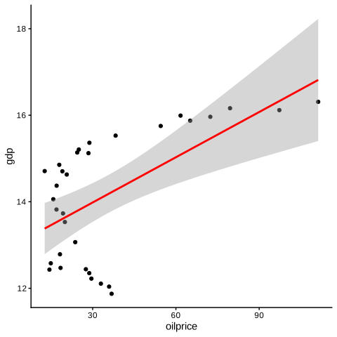
If you have noticed, we have many issues about this regression, such as the points that are not displayed randomly around the fitted line. We will discuss them in detail in the following chapters.
We first read the data.
import pandas as pd
# we read the data
data_p = pd.read_csv(
"alger.csv",
sep=';',  decimal=',')

# display the first 5 rows
data_p.head()| years | gdp | oilprice | gexp | inv |
|---|---|---|---|---|
| 80 | 143343 | 36.83 | 44016 | 54880 |
| 81 | 169035 | 35.93 | 57655 | 63044 |
| 82 | 181076 | 32.97 | 72445 | 71487 |
| 83 | 203580 | 29.55 | 84825 | 80319 |
| 84 | 231010 | 28.78 | 91598 | 87482 |
Then fit the model and display the results.
import numpy as np
from statsmodels.formula.api import ols
import pybroom as br
data_p['gdp']=np.log(data_p['gdp'])
m_p = ols('gdp ~ oilprice', data=data_p).fit()
m_p = m_p.summary2().tables[1]
m_p| Coef. | Std.Err. | t | P>|t| | [0.025 ] | ||
|---|---|---|---|---|---|---|
| Intercept | 12.9374632 | 0.3727419 | 34.708903 | 0.00000 | 12.1762227 | 13.6987038 |
| oilprice | 0.0348542 | 0.0086450 | 4.031697 | 0.00035 | 0.0171987 | 0.0525097 |
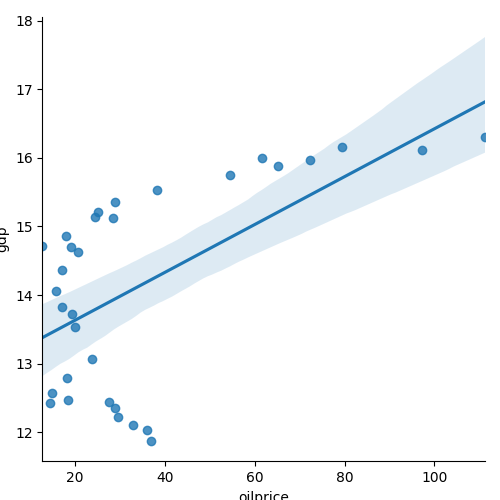
Figure 2.10: Linear regression with python