7.1 Concepts of Time Series

A time series is a sequence of data points collected over time, typically at regular intervals. Here are some key concepts associated with time series:

Time interval: The time interval is the time period between two consecutive observations in a time series. It can be seconds, minutes, hours, days, months, or years, depending on the frequency of data collection.
Time series data: Time series data refers to the set of observations collected at regular intervals over time. This data can be used to analyze and model trends, seasonality, and other patterns.
Trend: A trend in a time series is a long-term pattern of change in the data. It can be upward or downward, indicating an overall increase or decrease in the data over time.
Seasonality: Seasonality in a time series refers to regular patterns that occur at fixed intervals of time, such as daily, weekly, or monthly cycles.
Stationarity: A time series is stationary if its statistical properties, such as mean and variance, remain constant over time. Stationarity is important for time series analysis because it simplifies the modeling process and allows for more accurate predictions.
Autocorrelation: Autocorrelation in a time series refers to the correlation between the values of the series at different time points. A time series with high autocorrelation indicates that values at one time point are strongly related to values at nearby time points.
White noise: White noise is a time series where the data values are independent and identically distributed with a mean of zero and constant variance. White noise is often used as a benchmark for time series models because it has no discernible patterns or trends.
Forecasting: Forecasting is the process of using past data to predict future values in a time series. Forecasting can be done using various statistical and machine learning techniques, such as ARIMA, exponential smoothing, and neural networks.

7.1.1 Components of Times Series

The components of a time series can be broken down into four main parts: trend, seasonality, cyclical variation, and random variation. However, these components can be combined in additive model:

\[\begin{equation} y_t=Trend + Seasonality + Cyclical Variation + Random Variation \tag{7.1} \end{equation}\]

such that this model is linear where changes over time are consistently made by the same amount.

Or in multiplicative model:

\[\begin{equation} y_t=Trend \times Seasonality \times Cyclical Variation \times Random Variation \tag{7.2} \end{equation}\]

such that this model is nonlinear, such as quadratic or exponential. Changes increase or decrease over time.

7.1.1.1 Trend:

The trend component of a time series refers to a long-term pattern of change in the data. A trend can be positive (the values are increasing over time), negative (the values are decreasing over time), or flat (the values remain relatively constant over time). The trend can be modeled as a linear or non-linear function of time. A linear trend is a straight line that describes the overall direction and magnitude of change in the data over time, while a non-linear trend can take on any shape. the example of linear trend can be rewritten as follows:

\[\begin{equation} y_t=\beta_0+\beta_1t \tag{7.3} \end{equation}\]

where $y_t$ is the value of the time series at time $t$.

Using the the R package forcast the shape of such time series would be:

library(forecast)

# simulate the data
set.seed(1)
t <- 1:500
alpha <- 1
beta <- 0.005
theta <- 0.05
e <- rnorm(500,mean=0,sd=1)
ts <- alpha +beta*t + arima.sim(list(ma = theta), n = length(t))

# plot the time series
autoplot(ts)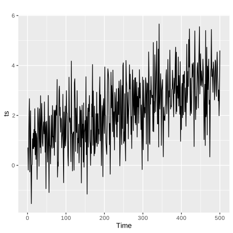

Figure 7.1: time series with linear trend

7.1.1.2 Seasonality

The seasonality component of a time series refers to regular patterns that occur at fixed intervals of time, such as daily, weekly, or monthly cycles. Seasonality can be modeled as a periodic function of time. For example, retail sales data may have a seasonal pattern that peaks during the holiday season and dips in the summer months. The seasonality component can be modeled using methods such as Fourier analysis or seasonal decomposition.

# Set the seed for reproducibility
set.seed(1)

# Simulate a seasonal time series with a quarterly frequency
ts_seasonal <- ts(rnorm(50*4, mean = 0, sd = 1), frequency = 4)

# Plot the time series
plot(ts_seasonal)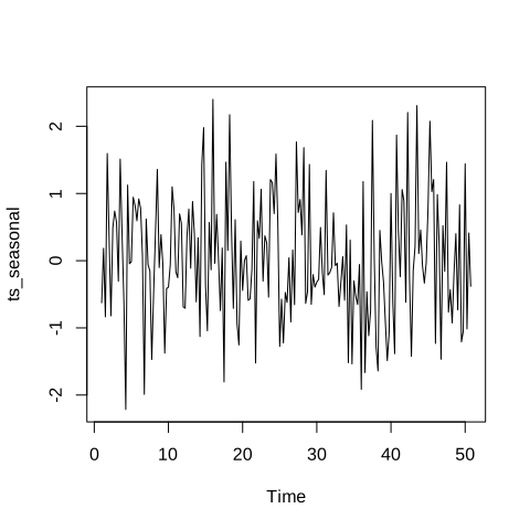

Figure 7.2: time series with a quarterly frequency

7.1.1.3 Cyclical variation

The cyclical component of a time series refers to patterns that occur over a longer time frame than seasonality, but are not as regular. Cyclical variation can be caused by business cycles, economic conditions, or other external factors. Unlike seasonality, cyclical variation does not have a fixed period. It can be modeled using methods such as spectral analysis or regression modeling.

set.seed(2)

t <-1:200
# Define the cyclical pattern
cycle <- sin(2*pi*t/12)

# Generate white noise
e <- rnorm(200, 0, 1)

# Generate the simulated time series
y <- cycle + e

# Plot the simulated time series
plot(y, type = "l")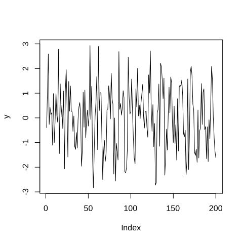

Figure 7.3: time series with a cyclical pattern

7.1.1.4 Random variation

The random component of a time series refers to the noise or error in the data that cannot be explained by the other components. It can be caused by measurement error, random fluctuations, or other factors. The random component is typically modeled as a white noise process, which has a mean of zero and constant variance over time.

we can combine the methods we discussed earlier. Here is an example code that generates a time series with all four components:

set.seed(11)

# Generate a time index
t <- 1:100

# Define the trend
trend <- 0.2*t

# Define the seasonal pattern
season <- rep(c(1, -1), length.out = 100/2)

# Define the cyclic pattern
cycle <- sin(2*pi*t/12)

# Generate white noise
e <- rnorm(100, 0, 1)

# Generate the simulated time series
full_y <- trend + season + cycle + e

# Plot the simulated time series
plot(full_y, type = "l")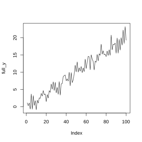

Figure 7.4: time series with all the components

In R:

We will take the above time series ts_seasonal and we will try to decompose the time series with the help of the R package stats.

# decompose the time series
decomp <- stats::decompose(ts_seasonal) 

# plot the decomposition results
plot(decomp)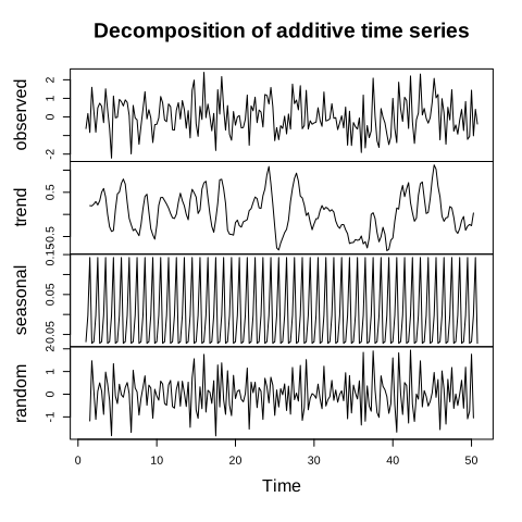

Figure 7.5: decomposition of additive time series in R

In Python:

We first move the data to python

if 'ts_seasonal_py' not in globals():
  ts_seasonal_py=r.ts_seasonal

To decompose a time series in Python, we are using the statsmodels package.

from statsmodels.tsa.seasonal import seasonal_decompose
import matplotlib.pyplot as plt 
result = seasonal_decompose(ts_seasonal_py, model='additive', period=4)
result.plot()

#> <Figure size 500x500 with 4 Axes>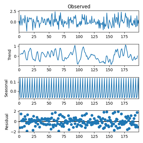

#plt.savefig("ts_seasonal_py.png")
plt.clf()
plt.close()

Figure 7.6: decomposition of time series in python

7.1.2 Stochactic process

Stochastic processes are mathematical models used to describe the evolution of random variables over time or space $(y_t; t=...,-2,-1,0,1,2,...)$ . In other words, a stochastic process is a collection of random variables indexed by time, or some other parameter, that describe a system whose evolution is subject to random influences.

Stochastic processes are used in a wide range of fields, including physics, engineering, finance, economics, and biology. Some examples of stochastic processes include Brownian motion, random walks, Poisson processes, and Markov processes.

The most most known properties in a stochastic processes are:

Markov property: A stochastic process has the Markov property(markov?) if the future evolution of the process depends only on its present state and not on its past history. Markov processes are widely used in modeling many phenomena, including stock prices, weather patterns, and biological systems. formally:

\[\begin{equation} Pr(Y_{t+1}=y|Y_0,Y_1,Y_2,..,Y_t)=Pr(Y_{t+1}=y|Y_t) \end{equation}\]

Martingales: A stochastic process is a martingale $Y_t$ if its expected value at any future time is equal to its current value, given its past history (in discrete_time):

\[\begin{cases} E(Y_t)=\mu \\ E(Y_{t+1}|Y_1,..,Y_t)=Y_t) \tag{7.4} \end{cases}\]

Martingales are used in finance and economics to model systems where the expected value of future gains or losses is zero.

7.1.3 White noise

A random sequence $Y_t$ is said to be a white noise process if it is independently and normally distributed with zero mean and finite variance.

\[\begin{align} &E(Y_t)=0 \\ &Var(Y_t)=\sigma^2 \\ &E(Y_tY_{t-i})=E(Y_{t-s}Y_{t-i-s})=0 \text{for all $i$ and $s$} \tag{7.5} \end{align}\]

7.1.4 Random walk

A basic example of a random walk is a person walking on a regular lattice so that moving by one unit to either right ($+1$) or left ($-1$) has equal probability.

Formally, if we have a 2-dimensional integer lattice with basis vectors $e_1\tbinom{1}{0}$, $e_2\tbinom{0}{1}$, and we have a stochastic process $Y_j$, $j=1,..,n$ such that $Pr(Y_j=e_1)=Pr(Y_j=-e_1)=Pr(Y_j=e_2)=Pr(Y_j=-e_2)=\tfrac{1}{4}$, then the random walk of n steps $Z_n$ will be determined as follows:

\[\begin{equation} Z_n=Z_0+\sum\limits_{j=1}^{n} Y_j \tag{7.6} \end{equation}\]

Where $Z_0$ is the position at step 0, and is commonly known as the drift parameter. If $Z_0=0$, then this formula could be rewritten:

\[\begin{equation} Z_n=Z_{n-1}+Y_n \tag{7.7} \end{equation}\]

Notice that $Y_n$ is a white noise since $E(Y_j)=0$

7.1.5 Autoregressive process AR

The intuitive idea behind this process is that the most effective predictors for a given variable are simply its own recent values. In a formal context, the expression for AR(p) can be articulated as follows::

\[\begin{equation} y_t=\phi_1y_{t-1}+\phi_2y_{t-2}+...+\phi_py_{t-p}+\varepsilon_t \tag{7.8} \end{equation}\]

Where $\varepsilon_t$ is a white noise (called also shocks), and $p$ is the order of regression.

Definition 7.1 (The lag operator) It takes the current value and gives the lagged value. $D^iy_t=y_{t-i}$

Properties of the lag operator:

The first difference:

\[\begin{align} \vartriangle Y_t&=Y_t-Y_{t-1} \\ &=Y_t-DY_t \\ &=(1-D)Y_t \end{align}\]

The second difference:

\[\begin{align} \vartriangle^2 Y_t&=(1-D)^2Y_t \\ &=(1-2D+D^2)Y_t \\ &=Y_t-2Y_{t-1}+Y_{t-2} \end{align}\]

For $\lvert\alpha\rvert <1$ :

\[\begin{equation} (1+\alpha D+\alpha D^2+..)Y_t=\tfrac{Y_t}{1-\alpha D} \end{equation}\]

Using the lag operator the above formula will be rewritten:

\[\begin{equation} (1-\phi_1D-\phi_2D^2-...-\phi_pD^p)Y_t=\varepsilon_t \tag{7.9} \end{equation}\]

The stationary of this process depends on the the parameters $\phi_1,..,\phi_p$. For simplicity, let us consider the first order Auto-regressive process $y_t=\phi_0+\phi_1 y_{t-1}+\varepsilon_t$. This process can be rewritten recursively in terms of $\varepsilon_t$ as follows (setting $\phi_0=0$ and $\phi_1=\phi$ for simplicity):

\[\begin{align} y_t&=\phi y_{t-1}+\varepsilon_t \\ &=\phi(\phi y_{t-2}+\varepsilon_{t-1})+\varepsilon_t \\ &=\phi^2y_{t-2}+\phi\varepsilon_{t-1}+\varepsilon_t \\ &=\phi^3y_{t-3}+\phi^2\varepsilon_{t-2}+\phi\varepsilon_{t-1}+\varepsilon_t \\ &............ \\ &=\varepsilon_{t}+\phi\varepsilon_{t-1}+\phi^{2}\varepsilon_{t-2}+... \end{align}\]

As observed, this process is entirely described using an infinite series of past white noise terms. In such instances, we characterize the process as invertible.

The mean of the process is equal to zero (since $\varepsilon_t$ is a white noise):

\[\begin{align} E(y_t)&=\overbrace{E(\varepsilon_{t})}^{=0}+\phi\overbrace{E(\varepsilon_{t-1})}^{=0}+\phi^{2}\overbrace{E(\varepsilon_{t-2})}^{=0}+... \\ &=0 \end{align}\]

And the variance will be:

\[\begin{align} Var(y_t)&=\overbrace{var(\varepsilon_{t})}^{=\sigma^2}+\phi^{2}\overbrace{Var(\varepsilon_{t-1})}^{=\sigma^2}+\phi^{4}\overbrace{Var(\varepsilon_{t-2})}^{=\sigma^2}+... \\ &=\sigma^2\overbrace{(1+\phi^2+\phi^4+...)}^{Geometric} \end{align}\]

If $|\phi|<1$ then the variance of the series will be reduced to the following:

\[\begin{equation} Var(y_t)=\frac{\sigma^2}{1-\phi^2} \end{equation}\]

In this case, we say that the AR process is stationary. In general, an $AR(p)$ process of order $p$ is stationary if the roots of the characteristic equation lie outside the unit circle. The characteristic equation for an $AR(p)$ process is given by:

\[\begin{equation} 1-\phi_1D-\phi_2D^2-...-\phi_pD^p=0 \tag{7.10} \end{equation}\]

7.1.6 Moving average process MA

The moving average process is a time series model that expresses each observation as a linear combination of past white noise error terms. Specifically, the $q-th$ order moving average process, denoted as MA(q), is defined as follows:

\[\begin{equation} y_t=\mu+\varepsilon_t-\theta_1\varepsilon_{t-1}-\theta_2\varepsilon_{t-2}-...-\theta_q\varepsilon_{t-q} \tag{7.11} \end{equation}\]

Where $\mu=E(y_t)$ is the mean of the time series.

\[\begin{equation} Y_t=\mu+(1-\theta_1D-\theta_2D^2-...-\theta_qD^q)\varepsilon_t \tag{7.12} \end{equation}\]

This process can also be expressed in relation to prior observations ($y_t$). To explain this, let’s examine the concept of a first-order moving average, denoted as $MA(1)$ (assuming $\mu=0$ for simplicity):

\[\begin{equation} y_t=\varepsilon_t-\theta_1\varepsilon_{t-1} \end{equation}\]

Shifting one time step backward results in:

\[\begin{equation} y_{t-1}=\varepsilon_{t-1}-\theta_1\varepsilon_{t-2} \end{equation}\]

Substituting the latter expression into the former one, we obtain:

\[\begin{align} y_t&=\varepsilon_t-\theta_1(y_{t-1}+\theta_1\varepsilon_{t-2}) \\ &=\varepsilon_t-\theta_1y_t-\theta_1^2\varepsilon_{t-2} \end{align}\]

Continuing this process, we obtain:

\[\begin{equation} y_t=\varepsilon_t-\theta_1y_{t-1}-\theta_1^2y_{t-2}-\theta_1^3y_{t-3}-..... \tag{7.13} \end{equation}\]

Similar to the condition applied to an Auto-regressive (AR) process, if the absolute value of the parameter $\theta_1$ in an Moving Average (MA) process is less than 1, we designate the process as invertible. In a more general context, an MA(q) process is deemed invertible when the roots of the associated characteristic equation exist outside the unit circle:

\[\begin{equation} 1-\theta_1D-\theta_2D^2-...-\theta_qD^q=0 \tag{7.14} \end{equation}\]

For invertibility, it is crucial that the roots of this characteristic equation do not fall within the unit circle. This condition ensures that the MA process can be effectively reconstructed from its observed values.

Regardless of the values of the parameters $\theta_i$, this process remains stationary at all times.

7.1.7 ARMA process

An ARMA (Auto-regressive Moving Average) model is a combination of Auto-regressive (AR) and Moving Average (MA) components. The general notation for an ARMA(p, q) model is as follows:

\[\begin{equation} y_t=\phi_1y_{t-1}+\phi_2y_{t-2}+...+\phi_py_{t-p}+\varepsilon_t-\theta_1\varepsilon_{t-1}-\theta_2\varepsilon_{t-2}-...-\theta_q\varepsilon_{t-q} \tag{7.15} \end{equation}\]

Alternatively, this can be expressed using the lag operator (D):

\[\begin{equation} Y_t=(\phi_1D+\phi_2D^2+...+\phi_pD^p)Y_t+(1-\theta_1D-\theta_2D^2-...-\theta_qD^q)\varepsilon_t \tag{7.16} \end{equation}\]

This notation emphasizes the dual characteristics of the model: the AutoRegressive (AR) component, representing the dependency of the current observation on its own past values, and the Moving Average (MA) component, signifying the influence of past white noise error terms on the present observation.

The parameters $\phi$ and $\theta$ are estimated from the data to fit the ARMA model to a given time series. The choice of p and q depends on the characteristics of the data and is often determined through statistical methods or model selection criteria.

7.1.8 Autocorrelation function ACF

The autocorrelation function (ACF) is a statistical tool used to quantify the correlation between the time series and its lagged values. In other words, it measures how the series is correlated with itself at different time lags. The ACF is a fundamental concept in understanding the temporal dependencies within a time series.

The autocorrelation function, denoted as $\gamma_k$, is defined as the correlation between the time series observations at time $t$ and the observations at time $t−k$, where $k$ is the lag, and is given by:

\[\begin{equation} \gamma_k=\frac{Cov(y_t,y_{t-k})}{\sqrt{Var(y_t)Var(y_{t-k})}}=\frac{Cov(y_t,y_{t-k})}{Var(y_t)} \tag{7.17} \end{equation}\]

The $\gamma_1$, for instance, will be (Assuming $\mu=0$):

\[\begin{align} \gamma_1&=\frac{Cov(y_t,y_{t-1})}{Var(y_t)} \\ &=\frac{E(y_ty_{t-1})}{Var(y_t)} \\ &=\frac{E[(\phi y_{t-1}+\varepsilon_t)y_{t-1}]}{Var(y_t)} \\ &=\frac{\phi E(y_{t-1}^2)+\overbrace {E(\varepsilon_ty_{t-1})}^{=0}}{Var(y_t)} \\ &=\frac{\phi Var(y_t) }{Var(y_t)} \\ &=\phi \tag{7.18} \end{align}\]

Similarly, the ACF(2) is given by:

\[\begin{align} \gamma_2&=\frac{Cov(y_t,y_{t-2})}{Var(y_t)} \\ &=\frac{E(y_ty_{t-2})}{Var(y_t)} \\ &=\frac{E[(\phi y_{t-1}+\varepsilon_t)y_{t-2}]}{Var(y_t)} \\ &=\frac{E[(\phi (\phi y_{t-2}+\varepsilon_{t-1})+\varepsilon_t)y_{t-2}]}{Var(y_t)} \\ &=\frac{\phi^2 E(y_{t-2}^2)+\phi \overbrace {E(\varepsilon_{t-1}y_{t-2})}^{=0}+\overbrace {E(\varepsilon_{t}y_{t-2})}^{=0}}{Var(y_t)} \\ &=\frac{\phi^2 Var(y_t) }{Var(y_t)} \\ &=\phi^2 \tag{7.19} \end{align}\]

Using the same procedure the $\gamma_k$ will be:

\[\begin{equation} \gamma_k=\phi^k \tag{7.20} \end{equation}\]

The findings indicate an exponential decrease in the parameter $\phi$ across previous periods. To clarify, in the context of a first-order auto-regressive model, the impact of past values diminishes as we delve further into the historical data.

Using the same logic, the autocorrelation function $\gamma_1$ of a $MA(1)$ $y_t=\varepsilon_t-\theta\varepsilon_{t-1}$ will be:

\[\begin{align} \gamma_1&=\frac{Cov(y_t,y_{t-1})}{Var(y_t)} \\ &=\frac{E(y_ty_{t-1})}{Var(y_t)} \\ &=\frac{E\big[(\varepsilon_t-\theta \varepsilon_{t-1})(\varepsilon_{t-1}-\theta \varepsilon_{t-2})\big]}{E\big[(\varepsilon_t-\theta \varepsilon_{t-1})^2\big]} \\ &=\frac{-\theta E(\varepsilon_{t-1}^2)}{E(\varepsilon_{t}^2)+\theta^2E(\varepsilon_{t-1}^2)}\quad{because}\quad\overbrace {E(\varepsilon_{t-i}\varepsilon_{t-j})}^{=0}\\ &=\frac{-\theta \sigma^2)}{\sigma^2+\theta^2\sigma^2} \\ &=\frac{-\theta}{1+\theta^2} \\ \tag{7.21} \end{align}\]

However, if we compute $\gamma_2$, and using the property of the white noise $E(\varepsilon_{t-i}\varepsilon_{t-j})=0$) we obtain the following:

\[\begin{align} \gamma_2&=\frac{Cov(y_t,y_{t-2})}{Var(y_t)} \\ &=\frac{E\big[(\varepsilon_t-\theta \varepsilon_{t-1})(\varepsilon_{t-2}-\theta \varepsilon_{t-3})\big]}{E\big[(\varepsilon_t-\theta \varepsilon_{t-1})^2\big]} \\ &=0 \tag{7.22} \end{align}\]

For the process $MA(1)$ the $\gamma_2=0$. This observation allows for a generalization: in an MA process of order $q$, the shocks occurring beyond $q$ periods have no influence on the process.

The visual representation of the autocorrelation function is termed a correlogram. In the illustration below, the contrast between $AR(1)$ and $MA(1)$ is evident. The first plot demonstrates the exponential decay of the parameters, while the second plot features a distinct singular spike (outside the confidence interval):

library(forecast)

# Set the seed for reproducibility
set.seed(123)

# Generate AR(1) time series
ar_series <- arima.sim(model = list(order = c(1, 0, 0), ar = 0.8), n = 100)

# Generate MA(1) time series
ma_series <- arima.sim(model = list(order = c(0, 0, 1), ma = 0.8), n = 100)

# Plot the correlogram
Acf(ar_series, main = "Correlogram for AR(1)")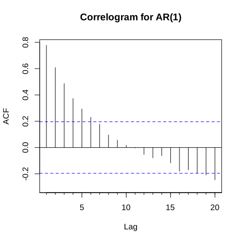

Figure 7.7: Correlogram for AR(1) and MA(1)

# Plot the correlogram
Acf(ma_series, main = "Correlogram for MA(1)")

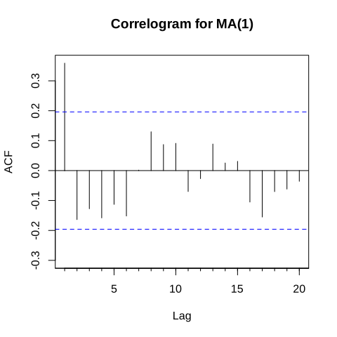
Figure 7.8: Correlogram for AR(1) and MA(1)

7.1.9 Partiall autocorrelation function PACF

The autocorrelation function has one drawback: the correlation it measures between $y_t$ and $y_{t-k}$ is not a direct one. Since $y_t$ is correlated with $y_{t-1}$, and $y_{t-1}$ is in its turn correlated with $y_{t-2}$, a part of what $\gamma_2$ captures is only the echo of the correlation already captured by $\gamma_1$. The partial autocorrelation function (PACF), denoted $\phi_{kk}$, removes these intermediate effects and keeps only the direct link between $y_t$ and $y_{t-k}$.

Formally, $\phi_{kk}$ is the coefficient attached to $y_{t-k}$ in the regression of $y_t$ on its first $k$ lags:

\[\begin{equation} y_t=\phi_{k1}y_{t-1}+\phi_{k2}y_{t-2}+...+\phi_{kk}y_{t-k}+\varepsilon_t \tag{7.23} \end{equation}\]

For the first lag nothing stands between $y_t$ and $y_{t-1}$, so the partial autocorrelation is simply equal to the autocorrelation:

\[\begin{equation} \phi_{11}=\gamma_1 \tag{7.24} \end{equation}\]

For the second lag, we subtract from $\gamma_2$ the part that transits through $y_{t-1}$:

\[\begin{equation} \phi_{22}=\frac{\gamma_2-\gamma_1^2}{1-\gamma_1^2} \tag{7.25} \end{equation}\]

We have shown for an $AR(1)$ process that $\gamma_k=\phi^k$ (7.20). Substituting this result into the above expression gives:

\[\begin{equation} \phi_{22}=\frac{\phi^2-\phi^2}{1-\phi^2}=0 \tag{7.26} \end{equation}\]

which is exactly what we expect. In an $AR(1)$ the only direct link is the one with the first lag, and everything beyond it is transmitted through $y_{t-1}$. More generally, the PACF of an $AR(p)$ process cuts off abruptly after the lag $p$, whereas its ACF decays slowly. For an $MA(q)$ process the roles are simply exchanged: the ACF cuts off after the lag $q$, while the PACF decays. This mirror image is the practical tool we use to guess the order of a process:

process	ACF	PACF
$AR(p)$	decays exponentially	cuts off after lag $p$
$MA(q)$	cuts off after lag $q$	decays exponentially
$ARMA(p,q)$	decays after lag $q$	decays after lag $p$

Let us plot the partial correlogram of the same two series simulated above, and compare it with their correlogram.

In R:

# Plot the partial correlogram
Pacf(ar_series, main = "Partial correlogram for AR(1)")

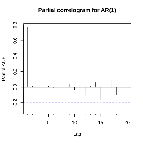
Figure 7.9: Partial correlogram for AR(1) and MA(1)

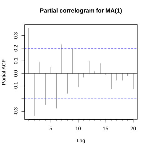
Pacf(ma_series, main = "Partial correlogram for MA(1)")

Figure 7.10: Partial correlogram for AR(1) and MA(1)

As announced, the $AR(1)$ shows a single spike at the first lag and nothing afterwards, while the $MA(1)$ shows a slow decay. This is the exact opposite of what the correlogram displayed.

In Python:

We first move the two series to python.

if 'ar_series_py' not in globals():
  ar_series_py = r.ar_series
if 'ma_series_py' not in globals():
  ma_series_py = r.ma_series

Then we use the function plot_pacf from the statsmodels package.

import matplotlib.pyplot as plt
from statsmodels.graphics.tsaplots import plot_pacf

fig, axes = plt.subplots(1, 2, figsize=(9, 3))
plot_pacf(ar_series_py, lags=20, ax=axes[0], title="AR(1)")

#> <Figure size 900x300 with 2 Axes>

plot_pacf(ma_series_py, lags=20, ax=axes[1], title="MA(1)")

#> <Figure size 900x300 with 2 Axes>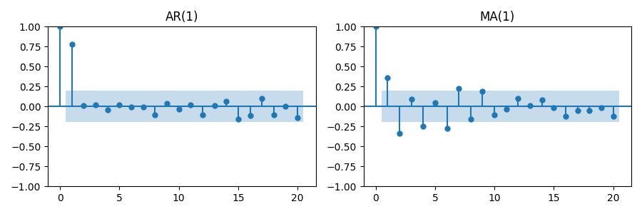

plt.tight_layout()
plt.savefig("pacf_py.png")
plt.clf()
plt.close()

Figure 7.11: partial correlogram in python

process	ACF	PACF
\(AR(p)\)	decays exponentially	cuts off after lag \(p\)
\(MA(q)\)	cuts off after lag \(q\)	decays exponentially
\(ARMA(p,q)\)	decays after lag \(q\)	decays after lag \(p\)