6.4 Binary response variable
Sometimes the dependent variable is constrained in two opposite states, one or yes, employed or unemployed..etc. For convenience we set such variable to 0 and 1. Since no constraints are made for the regressors values, any functional form \(\mathrm g(X, \beta)\) can not give exactly 0 or 1 as fitted values for the response variable. Therefore, we can still use the classical linear model but instead of the original response variable, we will use a latent (unobservable) variable \(y^*\) as a dependent variable \(y^*=X\beta+\varepsilon\) such that:
\[\begin{equation*} \begin{cases} y=1 \qquad y^*\geqslant c \\ y=0\qquad y^*<c \end{cases} \end{equation*}\]
Where \(c\) is a threshold that must be defined beforehand. However, since the latent variable \(y^*\) is unobservable, so we can use instead \(y^*-c\) as latent one and get rid of that threshold. Thus the original response variable and the latent variable will be related by the following:
\[\begin{equation} \begin{cases} y=1 \qquad y^*\geqslant 0 \\ y=0\qquad y^*<0 \end{cases} \tag{6.49} \end{equation}\]
As you we can see, \(y\) is not affected by the scale of \(y^*\), it is only related to its sign (positive or negative). Therefore, we can only check the conditional probability as follows:
\[\begin{align} Pr(Y=1|X)&=Pr(y^*\geqslant0|X) \\ &=Pr(X\beta+\varepsilon\geqslant0|X) \\ &=Pr(\varepsilon\geqslant -X\beta)\\ &=Pr(\varepsilon<X\beta)\\ &=F(X\beta) \tag{6.50} \end{align}\]
It remains to define the suitable distribution function \(F(.)\). The most used distributions in practice are the normal distribution \(\Phi(.)\), and the logistic distribution \(\Lambda(.)\), given in 6.3.1. Both of which are symmetric around zero mean. The difference is that the latter one has heavier tails so that it tends to produce larger probabilities than the former one for \(y=1\) when \(X\beta\) values are tiny, and small probabilities when \(X\beta\) values are high.
The marginal effect of some regressor is no longer the corresponding coefficient \(\beta\) like in the classical linear model, but instead it depends on all the regressors in the model:
If we still need to obtain the marginal effects, we can compute all the marginal effects for each value of \(X\), then take the average.
Whatever the distribution used, this model can be estimated by maximum likelihood method introduced in 3.3. The \(y\) of each single observation uses the Bernoulli probability so that it will be equal to 1 with probability \(F(X\beta)\) and 0 with the probability \(1-F(X\beta)\). Therefore, the likelihood of the data will be given by:
\[\begin{equation} L(\beta|data)=\prod_{i=1}^n F(x_i\beta)^{y_i}\big(1-F(x_i\beta)\big)^{1-y_i} \tag{6.51} \end{equation}\]
Then the log likelihood will be:
\[\begin{equation} LL(\beta|data)=\sum\limits_{i=1}^n\bigg[y_i ln \big(F(x_i\beta)\big)+(1-y_i) ln \big(1-F(x_i\beta)\big)\bigg] \tag{6.52} \end{equation}\]
The maximum likelihood estimator will be obtained by solving the following first derivatives:
\[\begin{equation} \frac{\partial LL}{\partial \beta}=\sum\limits_{i=1}^nx_i^t\Bigg[\frac{y_if(x_i\beta_{ML})}{F(x_i\beta_{ML})}-\frac{(1-y_i)f(x_i\beta_{ML})}{1-F(x_i\beta_{ML})}\Bigg] \tag{6.53} \end{equation}\]
If we use the logistic distribution, we will have \(F(x_i\beta)=\Lambda(X\beta)\) and \(f(x_i\beta)=\Lambda(x_i\beta)\big(1-\Lambda(x_i\beta)\big)\). Hence the above expression will be written:
\[\begin{align} \frac{\partial LL}{\partial \beta}&=\sum\limits_{i=1}^nx_i^t\Bigg[\frac{y_i\Lambda(x_i\beta_{ML})(1-\Lambda(x_i\beta_{ML}))}{\Lambda(x_i\beta_{ML})}-\frac{(1-y_i)\Lambda(x_i\beta_{ML})(1-\Lambda(x_i\beta_{ML}))}{1-\Lambda(x_i\beta_{ML})}\Bigg] \\ &=\sum\limits_{i=1}^nx_i^t\Bigg[y_i(1-\Lambda(x_i\beta_{ML}))-(1-y_i)\Lambda(x_i\beta_{ML})\Bigg] \\ &=\sum\limits_{i=1}^nx_i^t\Bigg[y_i-\Lambda(x_i\beta_{ML})\Bigg] \\ &=0 \tag{6.54} \end{align}\]
That model is also called The logit model
Similarly, if the normal distribution is used, the expression (6.53) thus will be rewritten:
\[\begin{align} \frac{\partial LL}{\partial \beta}&=\sum\limits_{i=1}^nx_i^t\Bigg[\frac{y_i\phi(x_i\beta_{ML})}{\Phi(x_i\beta_{ML})}-\frac{(1-y_i)\phi(x_i\beta_{ML})}{1-\Phi(x_i\beta_{ML})}\Bigg] \\ &=0 \tag{6.55} \end{align}\]
That model is called the probit model.
The logit model can also be rewritten as follows (we set \(P=Pr(Y=1|X)\) for simplification):
\[\begin{align*} P=\frac{exp(X\beta)}{1+exp(X\beta)}&\implies P+Pexp(X\beta)=exp(X\beta) \\ &\implies P=(1-P)exp(X\beta) \\ &\implies \frac{P}{1-P}=exp(X\beta) \\ &\implies log\Bigg(\frac{P}{1-P}\Bigg)=X\beta \end{align*}\]
The ratio \(\frac{P}{1-P}\) is called the odds. For instance, if \(odds=2\), this means the probability of choice \(y_i=1\) is twice than that of the alternative one.
This model can be seen as classical linear regression model where the response variable is the log odds.
For measuring the goodness of fit of this type of models,There exist bunch of measures. The most used ones are the following:
Cox and Snell ratio:
This one is given by (Allison and Paul.D):
\[\begin{equation} R^2_{cs}=1-\Bigg(\frac{L_{null}}{L_{fitted}}\Bigg)^{\frac{2}{n}} \tag{6.56} \end{equation}\]
Where \(L_{null}\) and \(L_{fitted}\) are the likelihood of the null model (fitted only with constant term) and the current model respectively.
McFadden ratio:
This one is given by (McFadden.D 1974):
\[\begin{equation} R^2_{cs}=1-\Bigg(\frac{LL_{fitted}}{LL_{null}}\Bigg)^{\frac{2}{n}} \tag{6.57} \end{equation}\]
For hypothesis testing, we can fit the two models, the restricted model and the unrestricted one, then we compute the likelihood ratio test introduced in 3.9.6:
\[\begin{equation} LR=-2(LL_{restricted}-LL_{unrestricted})\approx \chi^2_{(q)} \tag{6.58} \end{equation}\]
Where \(q\) is the number of constraint.
Example 6.2 We will use R to simulate 100 data points using logistic distribution and assuming the following relationship:
\[\begin{equation*} X\beta=0.1+1.5*x \end{equation*}\]
In R:
set.seed(1)

# create 100 samles from the normal distribution with mean 0 and sd 2
x <- rnorm(100,0,2)

# compute the predictor
x_beta <- 0.1 + 1.5*x

# compute the probability of that predictor with the logistic function
predictor <- 1/(1 + exp(-x_beta))

# generate the response variable
y <- rbinom(100, 1, predictor)

# put everything in data frame
df_binary <- tibble(y=y, x=x)

# display first rows
kbl(head(df_binary), booktabs = T, align = "c", col.names = gsub("[.]", " ", names(df_binary))) %>%
  kable_styling(latex_options = c("striped", "hold_position"),
full_width = F)| y | x |
|---|---|
| 0 | -1.2529076 |
| 1 | 0.3672866 |
| 0 | -1.6712572 |
| 1 | 3.1905616 |
| 1 | 0.6590155 |
| 0 | -1.6409368 |
To fit a linear regression model, we use the R function glm with the argument family set to binomial when we have a binary response variable. To use the logistic distribution we should set the link argument to logit, which is the default setting. And for the normal distribution, probit link should be specified instead.
[out]
[out] Call:
[out] glm(formula = y ~ x, family = binomial(link = "logit"), data = df_binary)
[out]
[out] Coefficients:
[out]             Estimate Std. Error z value Pr(>|z|)
[out] (Intercept)  -0.1730     0.2739  -0.632    0.528
[out] x             1.3080     0.2619   4.994 5.92e-07 ***
[out] ---
[out] Signif. codes:  0 '***' 0.001 '**' 0.01 '*' 0.05 '.' 0.1 ' ' 1
[out]
[out] (Dispersion parameter for binomial family taken to be 1)
[out]
[out]     Null deviance: 138.469  on 99  degrees of freedom
[out] Residual deviance:  85.231  on 98  degrees of freedom
[out] AIC: 89.231
[out]
[out] Number of Fisher Scoring iterations: 5
The interpretation of coefficients is made with the log odds. For instance, when \(x\) increases by one, the log adds of the first choice (vs the second choice) will increase by \(1.308\). However, it is better to interpret those coefficients in terms of odds. We can convert them to odds by exponentiation (with confidence intervals) as follows:
[out]                    OR     2.5 %   97.5 %
[out] (Intercept) 0.8411656 0.4834888 1.429837
[out] x           3.6987227 2.3408093 6.595086
Now the coefficient of \(x\) means that if \(x\) increases by \(1\), the probability of the first choice is \(3.7\) times than that of the second choice.
To test the significance of each individual parameter checking p-values. However, for testing the goodness of fit, we use the lrtest from the R package lmtest
[out] Likelihood ratio test
[out]
[out] Model 1: y ~ x
[out] Model 2: y ~ 1
[out]   #Df  LogLik Df  Chisq Pr(>Chisq)
[out] 1   2 -42.615
[out] 2   1 -69.235 -1 53.239  2.954e-13 ***
[out] ---
[out] Signif. codes:  0 '***' 0.001 '**' 0.01 '*' 0.05 '.' 0.1 ' ' 1
As we see, the model is highly significant with p-value equals to \(2.954e-13\).
We can plot the original and the fitted values using both link functions as follows:
ggplot(df_binary, aes(x, y))+
  geom_point()+
  stat_smooth(method="glm", se=FALSE, method.args = list(family=binomial))+
   stat_smooth(method="glm", se=FALSE, method.args = list(family=binomial(link="probit")), color="red")+
  xlab("x")+
  ylab("response variable")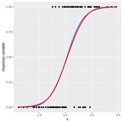
Figure 6.13: The logit model in R
We can also display the probabilities for each individual
[out]          1          2          3          4          5          6
[out] 0.14042624 0.57626019 0.08635697 0.98201817 0.66574831 0.08953779Now we will simulate the same data in Python. However, even we use the same seed we will not obtain exactly the same data due to the internel randomization process that is different. The logistic regression models can be easily implemented in statsmodels package.
import statsmodels.formula.api as smf
import numpy as np
from numpy import random
import pandas as pd
np.random.seed(1)
x=random.normal(0, 2, 100)
x_beta = 0.1 + 1.5*x
predictor = 1/(1 + np.exp(-x_beta))
y=random.binomial(1, predictor, 100)
df_binary_py = pd.DataFrame({"y":y, "x":x})

# fit with logit link
binary_logit_py = smf.logit("y~x", data=df_binary_py).fit()

# fit with probit link
binary_probit_py = smf.probit("y~x", data=df_binary_py).fit()[out] <class 'statsmodels.iolib.summary.Summary'>
[out] """
[out] Logit Regression Results
[out] ==============================================================================
[out] Dep. Variable: y No. Observations: 100
[out] Model: Logit Df Residuals: 98
[out] Method: MLE Df Model: 1
[out] Date: Thu, 17 Sept 2026 Pseudo R-squ.: 0.3694
[out] Time: 11:13:44 Log-Likelihood: -43.509
[out] converged: True LL-Null: -68.994
[out] Covariance Type: nonrobust LLR p-value: 9.372e-13
[out] ==============================================================================
[out] coef std err z P>|z| [0.025 0.975]
[out] ------------------------------------------------------------------------------
[out] Intercept 0.1612 0.267 0.604 0.546 -0.361 0.684
[out] x 1.2685 0.256 4.963 0.000 0.768 1.769
[out] ==============================================================================
[out] """As we see, the p-value of the log likelihood ratio is very tiny, indicating the high significance of the model.