5.1 Autoccorrelation
The term of Autoccorrelation refers here to the correlations among the disturbances. If some of the disturbances are correlated \(E(\varepsilon_t\varepsilon_s)\not= 0\) where \(t\not= s\), then we can suspect the presence of autoccorrelation. Note that the number of the correlated (pairs of) errors must be sufficient to create a certain pattern (of linear form) over time. Examples of some patterns are shown blow.
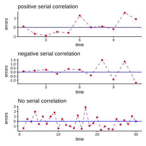
Figure 5.1: some patterns of correlations
Two points should be noted here:
- There is a slight difference between autocorrelation and serial correlation. The former describes the correlation in the same series, while, the latter can either occur in the same series or between two different series as in the SEM.
- There is a big difference between correlation and dependence. Two series are uncorrelated if they are not linearly related. But they can be by any other non-linear relationship. However, dependence can occur with any function of any form.
In application, the most encountered patterns are the ones expressed by an autoregressive process of order \(p\) known as \(AR(p)\).
\[\begin{equation} \varepsilon_t=\rho_1\varepsilon_{t-1}+\rho_2\varepsilon_{-2}+..+\rho_p\varepsilon_{t-p}+u_t \tag{5.1} \end{equation}\]
Where \(u_t\sim IID(0, \sigma^2_u)\), and orthogonal to every \(\varepsilon_{t-i}\) \(i=1,..,p\). Note that all the \(\rho_i\) must be \(-1\leqslant \rho_i\leqslant 1\) to maintain the errors around their zero mean. Otherwise, the process will be explosive, in which the influence of errors increases over time. Moreover, the constant term should not be included since the expectation of the errors is equal to zero by assumption.
What we learn from the equation (5.1) is that the error at the time \(t\) can be predicted by its p-lagged values. That is, they are no longer independently distributed. For instance, in models with quarterly time series, if we do not care about seasonal effects, we will have errors with \(4^{th}\) order of autocorrelation.
We start our investigation by the basic common case that face practitioners, the first-order autocorrelation expressed by:
\[\begin{equation} \varepsilon_t=\rho\varepsilon_{t-1}+u_t \tag{5.2} \end{equation}\]
Absolute values near \(1\) or \(-1\) signal a high degree of autocorrelation. If so, then a large part of the current error will be determined by the previous one. Positive values for \(\rho\) describe a positive autocorrelation, and negative ones negative autocorrelation. Note that the former case is more likely to occur in practice than the latter one.
5.1.1 The OLS properties under autocorrelation
First,let us check the unbiasedness in the multiple linear model:
\[\begin{align*} E\big(\widehat \beta\big) &= \beta+\big(X^tX\big)^{-1}X^t\overbrace{E(\varepsilon)}^{=0} \\ &=\beta \end{align*}\]
Which means that the unbiasedness does not require the assumption \(A4\). Even when the regressors are stochastic, the OLS estimators still consistent (but requires orthogonality assumption see 4.1.1).
Then, let us check the efficiency:
\[\begin{align} Var\big(\widehat \beta\big) &= \big(X^tX\big)^{-1}X^t\overbrace{E(\varepsilon\varepsilon^t)}^{=\Omega}X\big(X^tX\big)^{-1} \notag \\ &=\big(X^tX\big)^{-1}X^t\Omega X\big(X^tX\big)^{-1} \\ \tag{5.3} \end{align}\]
Where the matrix \(\Omega\not=\sigma^2I\).
To compute the elements of that matrix we have to express \(\varepsilon_t\) in terms of \(u_t\), since, by assumption, the latter ones are not correlated, and their variance is constant. Using the lag operator, the expression will be written:
\[\begin{equation*} \big(1-\rho L\big)\varepsilon_t=u_t \end{equation*}\]
Then the error \(\varepsilon_t\) will be:
\[\begin{align*} \varepsilon_t&=\frac{1}{1-\rho L}u_t \\ &= \big(1+\rho L+\rho^2 L^2+...\big)u_t \\ &= u_t+\rho u_{t-1}+\rho^2 u_{t-2}+... \end{align*}\]
Therefore, using \(\underset{i\not=j}{E\big(u_{t-i}u_{t-j}\big)}=0\) and \(\underset{i\not=j}{E\big(u_t^2\big)}=\underset{\forall i}{E}\big(u_{t-i}^2\big)=\sigma^2_u\), the variance will be:
\[\begin{equation} \sigma_{\varepsilon}^2=\frac{1}{1-\rho}\sigma_u^2 \tag{5.4} \end{equation}\]
Which is constant as it does not depend on time.
In the same way, the covariances will be determined as follows:
\[\begin{align*} E\big(\varepsilon_t\varepsilon_{t-1}\big)&=E\big[\big(\rho\varepsilon_{t-1}+u_t\big)\varepsilon_{t-1}\big] \\ &=\rho E\big(\varepsilon_{t-1}^2\big)+\overbrace{E\big(u_t\varepsilon_{t-1}\big)}^{=0} \\ &= \rho \sigma^2_{\varepsilon} \end{align*}\]
\[\begin{align*} E\big(\varepsilon_t\varepsilon_{t-2}\big)&=E\bigg[\big[\rho\big(\rho\varepsilon_{t-2}+u_{t-1}\big)+u_t\big]\varepsilon_{t-2}\bigg] \\ &=\rho^2 E\big(\varepsilon_{t-2}^2\big)+\rho\overbrace{E\big(\varepsilon_{t-2}u_{t-1}\big)}^{=0}+\overbrace{E\big(\varepsilon_{t-2}u_t\big)}^{=0} \\ &= \rho^2 \sigma^2_{\varepsilon} \\ \end{align*}\]
\[\begin{equation} E\big(\varepsilon_t\varepsilon_{t-h}\big)=\rho^h\sigma^2_{\varepsilon} \tag{5.5} \end{equation}\]
We see that these variances do not depend on time but, instead, on the number of lags between two errors.
Using the above results thus, the matrix \(\Omega\) can be written in terms of \(\rho\) as follows:
\[\begin{equation} \Omega=\sigma^2_{\varepsilon} \begin{pmatrix} 1&\rho&\rho^2&..&\rho^{n-1} \\ \rho&1&\rho&..&\rho^{n-2} \\ ..&..&..&..&.. \\ \rho^{n-1}&\rho^{n-2}&\rho^{n-3}&..&1 \end{pmatrix}=\sigma^2_{\varepsilon}P \tag{5.6} \end{equation}\]
Since some of the off-diagonal elements of \(\Omega\) are non-zero under autocorrelation, the variances computed from \(Var\big(\widehat\beta\big)=\sigma^2\big(X^tX\big)^{-1}\) underestimate the real ones in (5.3). That means, if we wrongly continue to use the classical variances to compute the classical statistic tests such as t-test and F-test, we would get incorrect results. Because in this case, those tests will be biased toward the alternative hypothesis. In other words, they tend to reject the null hypothesis more likely.
5.1.2 Causes of autocarrelation
Since the error term, \(\varepsilon_t\) is added in the model to replace all the possible unknown factors (regressors) that could affect the target variable, The causes of autocorrelation are likely related to the regressors in a certain way. The most common causes encountered in practice are the following:
5.1.2.1 Omitted relevant variables
Most of economic variables, say \(x_t\), are correlated with some of their lagged values, say \(x_{t-1}, x_{t-2},..,x_{t-p}\). If such variable is relevant for the model under study and mistakenly omitted, then by definition the error term will take charge of this autocorrelated variable, hence making this error term autocorrelated.
Suppose that we have the following DGP model:
\[\begin{equation*} y_t=\beta_1+\beta_2x_{2t}+\beta_3x_{3t}+u_t \end{equation*}\]
Where \(x_{3t}\) is assumed to be affected by the first order autocorrelation, and \(u_t\) follows the classical assumptions.
Suppose we wrongly assumed another model:
\[\begin{equation*} y_t=\alpha_1+\alpha_2x_{2t}+\varepsilon_t \end{equation*}\]
In the last model, the error term \(\varepsilon_t\) should contain the omitted variable \(x_{3t}\), say by the following function \(\varepsilon_t=\gamma x_{3t}=\nu_t\) (where \(\nu_t\) follows the classical assumptions). Now let us check the first order autocorrelation of \(\varepsilon_t\):
\[\begin{align*} E\big(\varepsilon_t\varepsilon_{t-1}\big)&=E\big[\big(\gamma x_{3t}+\nu_t\big)\big(\gamma x_{3,t-1}+\nu_{t-1}\big)\big] \\ &=\gamma^2E\big(x_{3t}x_{3,t-1}\big)+\gamma \overbrace{E\big(x_{3t}\nu_{t-1}\big)}^{=0}+\gamma \overbrace{E\big(\nu_{t}x_{3,t-1}\big)}^{=0}+ \overbrace{E\big(\nu_{t}\nu_{t-1}\big)}^{=0} \\ &=\gamma^2E\big(x_{3t}x_{3,t-1}\big) \\ &\not=0 \end{align*}\]
It should be noted that the omitted relevant variable not only causes autocorrelation but also biases the remaining regressors estimators, as discussed in chapter two, which is a more serious problem than this one.
5.1.2.2 Misspecification of the model
Suppose that real relationship between two variables is non-linear as follows (without constant term for simplification):
\[\begin{equation*} y_t=\beta_2x_{2t}^2+u_t \end{equation*}\]
Instead, we estimate the following linear model:
\[\begin{equation*} y_t=\alpha_2x_{2t}+\varepsilon_t \end{equation*}\]
Thus, the autocorrelation will be:
\[\begin{align*} E\big(\varepsilon_t\varepsilon_{t-1}\big)&=E\bigg[\big(y_t-\alpha_2x_{2t}\big)\big(y_{t-1}-\alpha_2x_{2,t-1}\big)\bigg] \\ &= E\bigg[\big(\overbrace{y_t-\beta_2x^2_{2t}}^{u_t}+\overbrace{\beta_2x^2_{2t}-\alpha_2x_{2t}}^{c_1}\big)\big(\overbrace{y_{t-1}-\beta_2x^2_{2,t-1}}^{u_{t-1}}+\overbrace{\beta_2x^2_{2,t-1}-\alpha_2x_{2,t-1}}^{c_2}\big)\bigg]\\ &= E\bigg[\big(u_t+c_1\big)\big(u_{t-1}+c_2\big)\bigg] \end{align*}\]
Since \(u_t\) is assumed to satisfy the classical assumptions, then:
\[\begin{align*} E\big(\varepsilon_t\varepsilon_{t-1}\big)&=\overbrace{E\big(u_t-u_{t-1}\big)}^{=0}+c_2\overbrace{E\big(u_t\big)}^{=0}+c_1\overbrace{E\big(u_{t-1}\big)}^{=0}+\overbrace{c_1c_2}^{\not=0} \\ &\not=0 \end{align*}\]
5.1.2.3 Biased measurement errors of some regressors.
Suppose that we have the following true model:
\[\begin{equation*} y_t=\beta x_{t}+u_t \end{equation*}\]
And suppose that we have estimated the following model with the regressor measured with errors as follows:
\[\begin{align*} y_t&=\alpha \tilde x_{t}+\varepsilon_t \\ \tilde x_{t}&=x_t+\nu_t \end{align*}\]
Then
\[\begin{align*} E\big(\varepsilon_t\varepsilon_{t-1}\big)&=E\bigg[\big(y_t-\alpha \tilde x_{t}\big)\big(y_{t-1}-\alpha \tilde x_{t-1}\big)\bigg] \\ &= E\bigg[\big(y_t-\alpha x_{t}-\alpha \nu_{t}\big)\big(y_{t-1}-\alpha x_{t-1}-\alpha \nu_{t-1}\big)\bigg] \\ &= E\bigg[\big(\overbrace{y_t-\beta x_t}^{=u_t}+\overbrace{\beta x_t-\alpha x_{t}}^{=c_1}-\alpha \nu_{t}\big)\big(\overbrace{y_{t-1}-\beta x_{t-1}}^{=u_{t-1}}+\overbrace{\beta x_{t-1}-\alpha x_{t-1}}^{=c_2}-\alpha \nu_{t-1}\big)\bigg] \\ &= E\bigg[\big(u_t+c_1-\alpha \nu_t\big)\big(u_{t-1}+c_2-\alpha \nu_{t-1}\big)\bigg] \\ & = ................................................. \\ &=c_1c_2 \\ &\not=0 \end{align*}\]
5.1.3 Testing for autocorrelation
To detect an autocorrelation of the first order, we can start first by representing the estimated model errors in the graph, where the errors in the vertical axis and either the time or the lagged values of errors in the horizontal axis. Therefore, if we can detect any particular pattern, then autocorrelation is present. The below graphs show one of autocorrelation, and also show its nature if positive or negative.
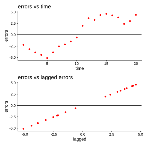
Figure 5.2: pattern of autocorrelation
Unfortunately, graphs alone cannot always give a reliable conclusion. Also does not help much with a higher order of autocorrelation. That is why statistical tests are needed.
5.1.3.1 Non parametric test:
Since errors, by their nature, have smaller values, we can only care about their signs \(+\) (or \(-\)) distribution whether randomly distributed or not.
That is what the Run test of randomness does, where Run is defined as the sequence of the symbol \(+\) (or \(-\)). The null hypothesis of no-autocorrelation holds if the runs (of symbol \(+\)) are normally distributed (if the sample size exceeds 25), or at least identically and independently distributed.
Let:
- \(m^+=\) number of (+).
- \(m^-=\) number of (-) (zero values will be also added here).
- \(r=\) number of runs.
Under the null hypothesis, the following test should be normally distributed with zero mean and variance equal to one:
\[\begin{equation} z=\frac{r-E(r)}{\sigma_r} \tag{5.7} \end{equation}\]
Where \(E(r)=\frac{2m^+m^-}{m^+m^-}+1\), \(\sigma_r^2=\frac{2m^+m^-(2m^+m^--m^+-m^-)}{(m^++m^-)^2(m^++m^--1)}+1\).
Therefore, we do not reject the null hypothesis with 95% confidence if:
\[\begin{equation} r \in \bigg[E\big(r\big)-1.96\sigma_r \quad , \quad E\big(r\big)+1.96\sigma_r\bigg] \tag{5.8} \end{equation}\]
5.1.3.2 Durbin Watson DW
It is the most popular test for autocorrelation introduced the first time by (Durbin.J and Watson 1950). This test is constrained to the first order correlation as described in (5.2). The null and the alternative hypotheses (derived from (5.2)) are:
\[\begin{equation} \begin{cases} H0: \rho=0 \quad no autocorrelation\\ H1: \rho\not=0 \quad autocorrelation \end{cases} \tag{5.9} \end{equation}\]
\(DW\) is derived from the distribution of the difference between two successive errors \((\varepsilon_t-\varepsilon_{t-1})\) with mean:
\[\begin{equation*} E\big(\varepsilon_t-\varepsilon_{t-1}\big)=0 \end{equation*}\]
And variance:
\[\begin{align*} Var\big(\varepsilon_t-\varepsilon_{t-1}\big)&=E\big(\varepsilon_t-\varepsilon_{t-1}\big)^2 \\ &=E\big(\varepsilon_t\big)^2+E\big(\varepsilon_{t-1}\big)^2-2cov\big(\varepsilon_t,\varepsilon_{t-1}\big) \\ &=2\sigma^2-2\rho\sigma^2 \\ &=2\sigma^2(1-\rho) \end{align*}\]
Where \(\rho=\frac{cov\big(\varepsilon_t,\varepsilon_{t-1}\big)}{\sigma^2}\) is the pearson correlation coefficient, which is unknown.
The idea behind this test is that, under autocorrelation, the difference between two successive errors tends to be very small. Using the estimated model, the DW is derived as follows:
\[\begin{equation} DW=\frac{\sum\limits^n_{t=2}\big(e_t-e_{t-1}\big)^2}{\sum\limits^n_{t=1}\big(e_t\big)^2} \tag{5.10} \end{equation}\]
It can also be expressed in terms of the estimated \(\widehat\rho=\frac{\sum e_te_{t-1}}{\sum e_t^2}\) such that we can determine the bound of this test:
\[\begin{align*} DW&=\frac{\sum\limits^n_{t=2}\big(e_t-e_{t-1}\big)^2}{\sum\limits^n_{t=1}\big(e_t\big)^2} \\ &= 2-2\frac{\sum e_te_{t-1}}{\sum e_t^2} \\ &= 2-2\widehat\rho \end{align*}\]
Therefore, we have three trivial cases:
- No autocorrelation: \(\widehat\rho=0\) \(\implies\) \(DW=2\).
- Perfect positive correlation: \(\widehat\rho=1\) \(\implies\) \(DW=0\).
- Perfect negative correlation: \(\widehat\rho=-1\) \(\implies\) \(DW=4\).
Durbin and Watson have tabulated two critical values, the lower bound \(dL\) and upper bound \(dU\) (Which they depend on the sample size n and the number of regressors \(k-1\)). They have shown that the distribution of DW swings between the distribution of \(dL\) and that of \(dU\) as in the following table:
| H1 | Reject H0 | do not reject H0 |
|---|---|---|
| \(\rho\not=0\) | d<dL \(\cup\) d>4-dL | dU<d<4-dU |
| \(\rho\) > \(0\) | d<dL | d>dU |
| \(\rho\) < \(0\) | d>4-dL | d<4-dU |
Or better explained as follows:
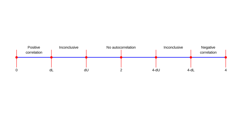
Figure 5.3: Durbin Watson statistic
However, the use of DW requires the following three conditions:
- Data must be ordered in time.
- The model must have a constant term.
- The lagged dependent variable must not be used as a regressor.
In time series, the first condition is crucial to compute the appropriate value for DW. Reordering the data will give different values, hence different conclusions. It is worthy to mention here that reordering data do not affect the main results such as the coefficient estimates, different statistic tests, intervals..etc. That is, only the DW will be affected and may give opposite results.
In general, we do not have the autocorrelation problem in cross-sectional data. But if it happens to have it, we can merely reorder the data randomly since ordering such data does not matter.
In nowadays, professionals do not much interested by DW, not only because of the inconclusive decisions showed above, but also because it requires many unrealistic conditions since almost the recent successful models are dynamics (lagged dependent variables in the regressors set).
For one side test, where the alternative hypothesis \(H1: \rho > 0\), the null hypothesis would be rejectd if \(DW < dL\), and will not if \(DW > dU\). The inconclusive region in this case is between \(dL\) and \(dU\).
5.1.3.3 Durbin h-test
When the lagged dependent variable is in the regressors set, DW tends to be closer to 2 even under autocorrelation, which may lead to opposite conclusion. That is why Durbin has proposed a modified version of its original test called Durbin h-test for that case. for instance, Suppose that the model being estimated is:
\[\begin{equation*} y_t=\beta_1+\alpha y_{t-1}+\beta_2x_{2t}+..+\beta_kx_{kt}+\varepsilon_t \end{equation*}\]
Thus, The Durbin h-test will be computed from the following formula:
\[\begin{equation} h=\bigg(1-\frac{DW}{2}\bigg)\sqrt{\frac{n}{n-nVar(\widehat\alpha)}} \tag{5.11} \end{equation}\]
Where \(\widehat\alpha\) is the OLS estimate of the lagged dependent variable.
Durbin has shown that this test, for large samples, follows the normal distribution under the null hypothesis. Therefore, if, for instance, \(h>1.645\) (in case of one sided test where \(H1:\rho>0\)), the null hypothesis of no correlation will be rejected.
5.1.3.4 Breusch Godfrey test BG-test
the interesting property of this test is the possibility to test higher order of autocorrelation without the restriction required in the case of \(DW\) test. Assuming that the order of autocorrelation is of \(p^{th}\) order as in (5.1), the null hypothesis of no correlation then will be:
\[\begin{align*} &H0: \rho_1=..=\rho_p=0 \\ &H1: \exists i \in [1,p]:\rho_i\not =0 \end{align*}\]
The procedure of this test can be summarized as follows:
- Step1: estimate the original model by the OLS method and obtaining the estimated residuals:
\[\begin{equation*} y_t=\widehat\beta_1+\widehat\beta_2x_{2t}+..+\widehat\beta_kx_{kt}+e_t+ \end{equation*}\]
- Step2: fit the following auxiliary regression:
\[\begin{equation*} e_t=\widehat\alpha_1+\widehat\alpha_2x_{2t}+..+\widehat\alpha_kx_{kt}+\widehat\rho_1 e_{t-1}+\widehat\rho_2e_{t-2}+..+\widehat\rho_pe_{t-p}+u_t \end{equation*}\]
- Step3: Compute the LM-test:
\[\begin{equation} LM=\big(n-p\big)R^2\sim \chi^2_{(p)} \tag{5.12} \end{equation}\]
Where \(R^2\) is computed from the auxiliary regression in step2.
This test has been derived in the same way as discussed in the subsection 3.9.5.
Larger values for this test lead to the rejection of the null hypothesis in favor of autocorrelation. It should be noted however that this test requires a large sample size to be accurate since its distribution is just an approximation of \(\chi^2\).
One might be confused about the reason behind adding the original regressors in the auxiliary regression. They are included to isolate the direct effect of each lagged error variable \(e_{t-i}\) from the indirect one of the regressors (as discussed in the section 3.8) that may exist in a case where the orthogonality condition is not perfect.
As we have seen, the BG-test requires that the order of autocorrelation being tested should be specified a priori. Since we can not know if the DGP errors are autocorrelated or not, we can try different values for the order \(p\) using the residuals of the estimated original model, then use one of the information criteria, such as Akaike or Schwarz, to select the best value.
5.1.3.5 Ljung-Box test
This test, like BG-test, can be used for higher order of autocorrelation. It is defined by:
\[\begin{equation} Q=n\sum\limits^p_{k=1}\frac{n+2}{n-k}\rho_k^2\sim\chi^2_{(p)} \tag{5.13} \end{equation}\]
Where \(\rho_k=\frac{\sum\limits ^n_{t=k+1}e_te_{t-k}}{\sum\limits ^n_{t=1}e_t^2}\) is the correlation coefficient between every two errors spaced out by \(k\) period.
Large values lead to the rejection of the null hypothesis of no correlation.
Example 5.1 Let us simulate two models in R, the first one with autocorrelated errors of the first order:
\[\begin{equation*} y_{1t}=1.2-0.5x2+0.2x3+e1 \end{equation*}\]
And the second with the third order:
\[\begin{equation*} y_{2t}=1.8+0.9x2-0.4x3+e2 \end{equation*}\]
In R:
set.seed(111)

# generate 50 errors of first order
e1 <- unclass(arima.sim(model=list(ar=0.9), n=50))

# generate errors of third order
e2 <- unclass(arima.sim(model=list(ar=c(0.8, -0.65, 0.5)), n=50))

# generate the regressors
x2 <- rnorm(50, 8, 3)
x3 <- rnorm(50,5,2)

# create the first model
y1 <- 1.2-0.5*x2+0.2*x3+e1

# create the second model
y2 <- 1.8+0.9*x2-0.4*x3+e2

# store everything in a data frame, then select 70 sample
df_corr <- tibble(y1=y1, y2=y2, x2=x2, x3=x3)
df_corr <- na.omit(df)
Now we will first fit the two models:
In R, it is straightforward to plot the resulted residuals as follows:
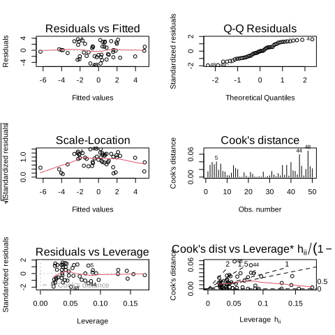
Figure 5.4: graphical detection of autocorrelation
As we see, the function plot has six plots for residuals.
- The first is the residuals vs the fitted values. With no autocorrelation, we expect the red line to be horizontal. The residuals should be orthogonal to the fitted values.
- The Normal Q-Q is used to check the normality of the residuals.
- The Scale-location plots the \(\sqrt{|residuals|}\) vs the fitted values.
- The Cook’s distance to check outliers.
- The Residuals vs leverage plots the standardized residuals vs the leverage observations, where leverage defines observations that have x-values far away from their corresponding means.
- The last one Cook’s dist vs leverage plots Cook’s distance vs \(\frac{leverage}{1-leverage}\)
For autocorrelation, we need the first plot.
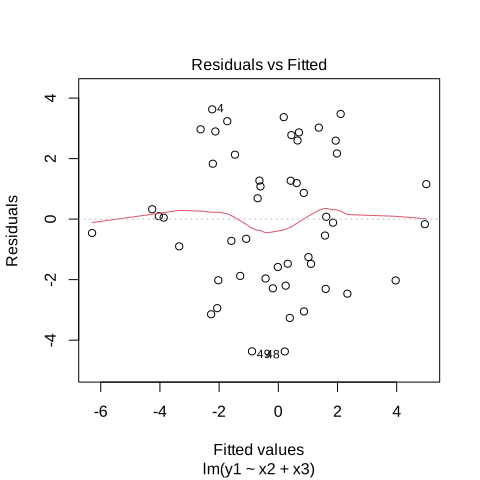
We see that the red line seems to be horizontal indicating no autocorrelation problem. That is why, in practice, we should not rely on plots to check assumptions, and we should get further investigation using statistic tests.
Non parametric test: To apply this test we call the package snpar. we can specify the alternative hypothesis from three choices, two.sided (the default), less, and greater
[out]
[out]   Approximate runs rest
[out]
[out] data:  mod1$residuals
[out] Runs = 12, p-value = 6.312e-05
[out] alternative hypothesis: two.sided
Since p-value is closer to zero, the autocorrelation is present.
DW:
[out]  lag Autocorrelation D-W Statistic p-value
[out]    1       0.8064026     0.3469645       0
[out]  Alternative hypothesis: rho != 0
As expected, the DW has detected the autocorrelation (\(p-value=0\)). By default this function uses two-sided hypothesis, but we can test the positive correlation as follows:
[out]  lag Autocorrelation D-W Statistic p-value
[out]    1       0.8064026     0.3469645       0
[out]  Alternative hypothesis: rho > 0
However, if we test the negative correlation:
[out]  lag Autocorrelation D-W Statistic p-value
[out]    1       0.8064026     0.3469645       1
[out]  Alternative hypothesis: rho < 0
As we see the test did not reject the null hypothesis of no correlation.
BG-test: This test can be used for both models, mod1 and mod2. It is provided from the R package lmtest.
For the first model, it should give the same result as with DW
[out]
[out]   Breusch-Godfrey test for serial correlation of order up to 1
[out]
[out] data:  mod1
[out] LM test = 36.105, df = 1, p-value = 1.87e-09
As expected, we get the same result. Now let us check the second model:
[out]
[out]   Breusch-Godfrey test for serial correlation of order up to 3
[out]
[out] data:  mod2
[out] LM test = 39.105, df = 3, p-value = 1.649e-08
The test detected autocorrelation of order 3.
Ljung Box:
[out]
[out]   Box-Ljung test
[out]
[out] data:  mod1$residuals
[out] X-squared = 34.505, df = 1, p-value = 4.252e-09
This test also detected autocorrelation.
We first move the data to python
Non parametric test:
To implement this test, we use statsmodels package
import statsmodels.formula.api as smf
from statsmodels.sandbox.stats.runs import runstest_1samp

# first fit the model
mod1_py = smf.ols("y1~x2+x3", data=df_corr_py).fit()
mod2_py = smf.ols("y2~x2+x3", data=df_corr_py).fit()

# apply the runs test for mod1_py
runstest_1samp(mod1_py.resid, correction=False)
[out] (-16.95806340328209, 1.6778384824256798e-64)Unlike R function runs.test, this python function produces both the z-score value along with the p-value in a tuple. Since the p-value is less than \(0.05\), the autocorrelation is present (with 95%of confidence).
DW:
For the first model:
[out] 0.5687823894602889Unfortunately, this function does not provide the corresponding p-value. Thus, we should compare this value to the corresponding (\(n=50\), \(k=2\)) \(dL=1.285\) and \(dU=1.445\) provided here. Since the computed \(DW=0.56878\) is less than \(dL=1.285\), then a positive autocorrelation is present.
BG-test:
We test the second model:
from statsmodels.stats.diagnostic import acorr_breusch_godfrey
acorr_breusch_godfrey(mod2_py, nlags=3)
[out] (530.2714249123129, 1.3122875194913669e-114, 374.03855780929354, 1.4843792885607338e-162)The first two values are the LM statistic value and its p-value, and the last ones are F statistic and its p-value. Both p-values are less than \(0.05\) indicating the presence of autocorrelation of order 3.
Ljung-Box:
We use the second model:
from statsmodels.stats.diagnostic import acorr_ljungbox
acorr_ljungbox(mod2_py.resid, lags=[3], return_df=True)
[out] lb_stat lb_pvalue
[out] 3 347.406294 5.436075e-75This test also rejected the null hypothesis of no autocorrelation in favor of autocorrelation of order 3.
5.1.4 Estimation under autocorrelation
Actually, the best way to deal with autocorrelation is by searching for its causes and fix the problem from the beginning. For instance, the investigator can try different specifications for their model, or looking for any missing relevant variables, ..etc.
However, if all those attempts failed, we can use other methods to estimate the model under autocorrelation. In the following subsection, we will illustrate the most important ones, Transformed variables, Generalized least squares GLS, Newey west, Generalized method of moments GMM, and Maximum likelihood MM.
5.1.4.1 Transformed variables
For simplicity, let us assume having the first-order autocorrelation as in (5.2). Since the OLS method can be used only with white noise errors, we can include the term \(u_t\) instead of \(\varepsilon_t\) by pre multiplying the shifted model (by one lag) by the \(\rho\) in the first step, then subtracting from the original model in the next step as follows:
\[\begin{equation} y_t-\rho y_{t-1}=\beta_1\big(1-\rho\big)+\beta_2\big(x_{2t}-\rho x_{2,t-1}\big)+..+\beta_k\big(x_{kt}-\rho x_{k,t-1}\big)+\overbrace{\varepsilon_t-\rho\varepsilon_{t-1}}^{u_t} \tag{5.14} \end{equation}\]
As the errors \(u_t\) now are free of autocorrelation, we can apply the OLS method using the transformed variables \((y_t-\rho y_{t-1})\) and \((x_{kt}-\rho x_{k,t-1})\) instead of the original ones.
This transformation is called Quasi difference transformation, which is analogous to the first difference method where \(\rho=1\).
To get this transformation in matrix form, we should premultiply the original model by the matrix \(P\) as follows:
\[\begin{align*} Py&=PX\beta+\overbrace{P\varepsilon}^{=u} \\ &=PX\beta+u \end{align*}\]
Where the matrix \(P\) is given by:
\[\begin{equation} \underset{(n-1,n)}{P}= \begin{pmatrix} -\rho&1&0&..&0 \\ 0&-\rho&1&..&0 \\ ..&..&..&..&..& \\ 0&0&..&-\rho&1 \end{pmatrix} \tag{5.15} \end{equation}\]
And the matrices \(Py\) and \(PX\) are given by:
\[\begin{align*} Py&= \begin{pmatrix} y_2-\rho y_1 \\ .. \\ y_n-\rho y_{n-1} \end{pmatrix} \\ PX&=\begin{pmatrix} 1-\rho&x_{22}-\rho x_{21}&..&x_{k2}-\rho x_{k1} \\ ..&..&..&.. \\ 1-\rho&x_{2n}-\rho x_{2,n-1}&..&x_{kn}-\rho x_{k,n-1} \end{pmatrix} \end{align*}\]
Notice that we have lost one observation with this method.
For testing any linear hypothesis, we can still use the classical F-test for the transformed model as follows:
\[\begin{equation*} F^c_{(q,n-k)}=\frac{\bigg(R\widehat\beta-r\bigg)^t\bigg[s^2R\bigg(X^{*t}X^{*}\bigg)^{-1}R^t\bigg]\bigg(R\widehat\beta-r\bigg)}{q} \end{equation*}\]
Where \(X^{*}=PX\), and \(s^2=\frac{e^{*t}e^*}{n-k}\) where \(e^*=y^*-X^*\widehat\beta\).
The serious caveat of this method is that it depends on the parameter \(\rho\), which is in most cases unknown. However, we will shortly introduce some other alternatives used often in practice.
In R:
Let us call again the example 5.1, but this time, we will generate a population with 100 samples than take out 50 samples respecting the order to save autocorrelation.
set.seed(111)

# generate 50 errors of first order
e1 <- unclass(arima.sim(model=list(ar=0.9), n=100))

# generate errors of third order
e2 <- unclass(arima.sim(model=list(ar=c(0.8, -0.65, 0.5)), n=100))

# generate the regressors
x2 <- rnorm(100, 8, 3)
x3 <- rnorm(100,5,2)

# create the first model
y1 <- 1.2-0.5*x2+0.2*x3+e1

# create the second model
y2 <- 1.8+0.9*x2-0.4*x3+e2

# store everything in a data frame, then select 51 samples
df <- tibble(y1=y1, y2=y2, x2=x2, x3=x3)

df_corr2 <- df[30:80,]
We fit OLS model first, then check the autocorrelation by DW. But before that, we should first fix an issue resulted when we generated the data so that the two variables \(y1\) and \(y2\) are times series object tsp. we should then remove this attribute using a package called labelled
[out] tibble [51 × 4] (S3: tbl_df/tbl/data.frame)
[out]  $ y1: num [1:51] -2.494 -4.42 -3.294 -0.438 0.719 ...
[out]  $ y2: num [1:51] 9.68 10.84 9.61 8.84 7.06 ...
[out]  $ x2: num [1:51] 9.12 9.68 7.99 8.55 7.22 ...
[out] $ x3: num [1:51] 7.379 1.846 -0.606 4.61 5.491 ...[out]
[out] Durbin-Watson test
[out]
[out] data: model_ar1
[out] DW = 0.39387, p-value = 2.049e-13
[out] alternative hypothesis: true autocorrelation is greater than 0Indeed, the model is autocorrelated. So since we know that \(\rho=0.9\) (the data generated using this value), we can go ahead and fit a model with the transformed variables.
# create the transformed variables

df <- transform(df_corr2,
                lagy1=dplyr::lag(y1),
                lagx2=dplyr::lag(x2),
                lagx3=dplyr::lag(x3))

# remove the missing values
df <- na.omit(df)
df <- transform(df,
                dy1=y1-lagy1,
                dx2=x2-lagx2,
                dx3=x3-lagx3)

# remove the intermediate variables
df <- within(df, rm(lagy1, lagx2, lagx3))

# fit the model
model_transformed <- lm(dy1~dx2+dx3, df)
lmtest::dwtest(model_transformed)
[out]
[out] Durbin-Watson test
[out]
[out] data: model_transformed
[out] DW = 2.007, p-value = 0.568
[out] alternative hypothesis: true autocorrelation is greater than 0As we see the DW value is closer to \(2\) indicating no autocorrelation with p-value much larger than \(0.05\). We can also check the plot:
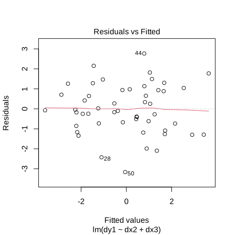
Figure 5.5: The residuals of the transformed model in R
The line now is flat. We see in the plot some points flagged with numbers. Those points are outliers and will be discussed in more detail later on.
The last thing we should know about this model is that the coefficients are now completely different from those of the original model. Here each coefficient is the marginal effect of the transformed associated regressor on the transformed response variable.
In Python:
First, we move the data to the Python workspace.
As we did in R, we will add the transformed variables to the data frame:
# transform the variables
df_corr2_py["dy1"] = df_corr2_py["y1"] - 0.9*df_corr2_py["y1"].shift(-1)

df_corr2_py["dx2"] = df_corr2_py["x2"] - 0.9*df_corr2_py["x2"].shift(-1)

df_corr2_py["dx3"] = df_corr2_py["x3"] - 0.9*df_corr2_py["x3"].shift(-1)

# drop the missing values
df_corr2_py.dropna(inplace=True)
Then, we fit the model and display the DW value.
import statsmodels.formula.api as smf
from statsmodels.stats.stattools import durbin_watson

# fit the model
mod_ar_py = smf.ols("dy1~dx2+dx3", data=df_corr2_py).fit()
durbin_watson(mod_ar_py.resid)
[out] 1.97195119623880145.1.4.2 Generalized least squares GLS
Let our model be:
\[\begin{equation} y=X\beta+\varepsilon \tag{5.16} \end{equation}\]
And let us denote the estimator that we are searching for \(\beta_{GLS}\). Since any competitor estimator must be a linear function of the dependent variable \(y\), then this estimator should also satisfy this restriction:
\[\begin{equation*} \beta_{GLS}=\underset{(k,n)}{A}y \end{equation*}\]
Where \(A\) is a non singular matrix.
Substituting (5.16) into the formula above, we get:
\[\begin{equation} \beta_{GLS}=AX\beta+A\varepsilon \tag{5.17} \end{equation}\]
Remember that we already have the OLS estimator that still unbiased under autocorrelation but not efficient. Therefore, to be a competitor, the new one \(\beta_{GLS}\) must also be unbiased:
\[\begin{align*} E\big(\beta_{GLS}\big)&=AX\beta+A\overbrace{E\big(\varepsilon\big)}^{0} \\ &=AX\beta \end{align*}\]
As we see, the estimator is unbiased if \(AX=I\).
Under this condition, the expression (5.17) will be:
\[\begin{equation*} \beta_{GLS}=\beta+A\varepsilon \end{equation*}\]
hence, the variance will be:
\[\begin{align} Var\big(\beta_{GLS}\big)&= E\bigg[\big(\beta_{GLS}-\beta\big)\big(\beta_{GLS}-\beta\big)^t\bigg] \notag \\ &= E\bigg[\big(A\varepsilon\big)\big(A\varepsilon\big)^t\bigg] \notag \\ &= AE\big(\varepsilon\varepsilon^t\big)A^t \notag \\ &=A\Omega_{\varepsilon}A^t \tag{5.18} \end{align}\]
Where the diagonal elements of \(\Omega_{\varepsilon}\) are the individual variances, and the off-diagonal ones are the covariances. Under autocorrelation thus, some of the off-diagonal elements are different from zero such that \(\Omega_{\varepsilon}\not=\sigma_{\varepsilon}^2I\).
Since the best estimator should have the minimum variance, we have to minimize the trace of the \(Var\big(\beta_{GLS}\big)\) matrix, indeed under the condition \(AX=I\) used to compute it. That is:
\[\begin{equation} \begin{cases} Min: \quad Tr\big(A\Omega_{\varepsilon}A^t\big) \\ s.t \quad \quad AX=I \end{cases} \tag{5.19} \end{equation}\]
As usual, we use the Lagrange function to solve this problem:
\[\begin{equation*} L = Tr\bigg(A\Omega_{\varepsilon }A^t\bigg)-Tr\bigg[\lambda^t\big(AX-I\big)\bigg] \end{equation*}\]
Where \(\lambda\) is a \((k\times k)\) multiplier matrix
Using the trace operator properties, we have:
\[\begin{equation*} Tr\bigg(A\Omega_{\varepsilon }A^t\bigg)=Tr\bigg(A^tA\Omega_{\varepsilon }\bigg) \end{equation*}\]
\[\begin{align*} Tr\bigg(\lambda^tAX\bigg)&=Tr\bigg(\lambda^tAX\bigg)^t \\ &=Tr\bigg(X^tA^t\lambda\bigg)\\ &=Tr\bigg(A^t\lambda X^t\bigg) \end{align*}\]
After substituting those results, the above Lagrange function will be:
\[\begin{equation*} L = Tr\bigg(A^tA\Omega_{\varepsilon }\bigg)-Tr\bigg(A^t\lambda X^t\bigg)+Tr\bigg(\lambda^t\bigg) \end{equation*}\]
The differentiation equation then will be:
\[\begin{align*} dL&=Tr\bigg(dA^tA\Omega_{\varepsilon }\bigg)+Tr\bigg(A^tdA\Omega_{\varepsilon }\bigg)-Tr\bigg(dA^t\lambda X^t\bigg) \\ &=Tr\bigg[dA^t\big(2A\Omega_{\varepsilon }-\lambda X^t\big)\bigg] \end{align*}\]
Setting this equation to zero, we get:
\[\begin{align*} dL=0 \quad & \implies \quad 2A\Omega_{\varepsilon}-\lambda X^t=0 \\ &\implies \quad 2A\Omega_{\varepsilon}=\lambda X^t \end{align*}\]
Postmultiplying both sides of the last equation by \(\Omega_{\varepsilon}^{-1}X\) to allow the use of the condition \(AX=I\) as follows:
\[\begin{align*} 2A\overbrace{\Omega_{\varepsilon}\Omega_{\varepsilon}^{-1}}^{=I}X=\lambda X^t\Omega_{\varepsilon}^{-1}X \quad &\implies \quad 2\overbrace{AX}^{=I}=\lambda X^t\Omega_{\varepsilon}^{-1}X \\ &\implies \quad \lambda=2\bigg(X^t\Omega_{\varepsilon}^{-1}X\bigg)^{-1} \end{align*}\]
Substituting this result into \(2A\Omega_{\varepsilon}=\lambda X^t\), we get:
\[\begin{equation*} 2A\Omega_{\varepsilon}=2\bigg(X^t\Omega_{\varepsilon}^{-1}X\bigg)^{-1} X^t \quad \implies \quad A=\bigg(X^t\Omega_{\varepsilon}^{-1}X\bigg)^{-1}X^t\Omega_{\varepsilon}^{-1} \end{equation*}\]
Finally, the GLS estimator will be given by:
\[\begin{equation} \begin{cases} \beta_{GLS}=\big(X^t\Omega_{\varepsilon}^{-1}X\big)^{-1} X^t\Omega_{\varepsilon}^{-1}y \\ Var(\beta_{GLS})=\big(X^t\Omega_{\varepsilon}^{-1}X\big)^{-1} \tag{5.20} \end{cases} \end{equation}\]
It should be noted that this method not only gives efficient estimator under autocorrelation, but also under heteroskedasticity (that will be discussed later).
For instance, if we have a first order autocorrelation, the matrix \(\Omega_{\varepsilon}\) (using (5.4) and (5.5)) will be:
\[\begin{align} \Omega_{\varepsilon}&=\frac{\sigma_u^2}{1-\rho} \begin{pmatrix} 1&\rho&\rho^2&..&\rho^{n-1} \\ \rho&1&\rho&..&\rho^{n-2} \\ ..&..&..&..&.. \\ \rho^{n-1}&\rho^{n-2}&\rho^{n-3}&..&1 \end{pmatrix} \notag \\ &=\sigma^2_u\bigg(\frac{\Omega_{\rho}}{1-\rho}\bigg) \notag \\ &=\sigma^2_u\Omega \tag{5.21} \end{align}\]
Where \(\sigma^2_u\) is the variance of a white noise (which is a constant term), so we can ignore the subscript \(u\), and \(\Omega=\frac{\Omega_{\rho}}{1-\rho}\).
Using the matrix algebra, the inverse of the matrix \(\Omega_{\varepsilon}\) is given by:
\[\begin{align} \Omega_{\varepsilon}&=\frac{1}{\sigma^2} \begin{pmatrix} 1&-\rho&0&..&..&0 \\ -\rho&1+\rho^2&-\rho&..&..&0 \\ 0&-\rho&1+\rho^2&-\rho&..&0 \\ ..&..&..&..&..&0 \\ 0&0&0&..&1+\rho^2&-\rho \\ 0&0&0&..&-\rho&1 \end{pmatrix} \notag \\ &=\frac{1}{\sigma^2}\Omega^{-1} \tag{5.22} \end{align}\]
Substituting this result into the GLS formula (5.20), the unknown term \(\sigma^2\) will be dropped and the \(\beta_{GLS}\) will depend only on one unknown parameter (\(\rho\)) (in case of the first order autocorrelation):
\[\begin{align*} \beta_{GLS}&=\big(X^t\frac{1}{\sigma^2}\Omega^{-1}X\big)^{-1} X^t\frac{1}{\sigma^2}\Omega^{-1}y \\ &=\big(X^t\Omega^{-1}X\big)^{-1} X^t\Omega^{-1}y \end{align*}\]
Consequently, if the investigator can correctly define the value of \(\rho\), then GLS estimates will be straightforward.
There exists some connection between this estimator and the previous one if we can find a matrix \(P_2\) such that \(\Omega^{-1}=P_2^tP_2\). It turns out that this matrix exists, and is given by:
\[\begin{equation*} \underset{(n,n)}{P_2}=\begin{pmatrix} \sqrt{1-\rho^2}&0&..&..&..\\ -\rho&1&..&..&..\\ ..&-\rho&1&-\rho&..\\ ..&..&..&..&..\\ ..&..&..&-\rho&1 \end{pmatrix} \end{equation*}\]
As we see, this matrix is slightly different from the matrix \(P\) used for transformation. Because in the previous method, we have lost the first observation after that transformation. The GLS method, in contrast, keeps the first observation but corrected by the factor \(\sqrt{1-\rho^2}\). Consequently, the two methods will likely give different estimates in small samples.
This methods suffers from the same caveat as the previous one, the unknown value of \(\rho\). However, practitioner have proposed several techniques to estimate this parameter, which are grouped under one big title called Feasible general least squares FGLS. We will introduce the most important one that is often used in practice which is called Restricted maximum likelihood.
In R:
To fit autocorrelated model in R, We will use the R package nlme that has a function called gls. This function uses two method to estimate parameters: the maximum likelihood named ML under the argument method, or the restricted log likelihood named REML.
We set the argument fixed to TRUE in gls function since the value \(0.9\) (in corAR1) for \(\rho\) is known.
library(nlme)
# ols model
mod_ols <- lm(y1~x2+x3, data=df_corr2)

# gls model
mod_gls <- gls(y1~x2+x3, data=df_corr2, correlation = corAR1(0.9, form = ~1, fixed=TRUE))
Let us compare the coefficients and the standard errors of the GLS and the OLS methods.
ols_gls <- tibble(coef=names(mod_ols$coefficients),
       c_ols=mod_ols$coefficients,
       c_gls=mod_gls$coefficients,
       std_ols=summary(mod_ols)$coefficients[, 2],
       std_gls=sqrt(diag(summary(mod_gls)$varBeta)))
ols_gls
[out] # A tibble: 3 × 5
[out] coef c_ols c_gls std_ols std_gls
[out] <chr> <dbl> <dbl> <dbl> <dbl>
[out] 1 (Intercept) 1.91 0.762 1.12 1.52
[out] 2 x2 -0.556 -0.470 0.122 0.0543
[out] 3 x3 0.250 0.252 0.128 0.0543As we see, the coefficients of the two models are less or more closer to each other(except for the intercept). Whereas, the standard errors of GLS are much smaller than those of OLS method (except also for the intercept), which means more accurate estimates and free of autocorrelation. However, we have obtained a high accuracy because we know the exact value of \(\rho\), which is not the case in practice so that this value should be estimated.
In Python:
In Python, we will use the GLS function from statsmodels package. But before that we should firs compute the covariance function by hand using the toeplitz function from scipy package.
from scipy.linalg import toeplitz
# create the covariance matrix of errors using the value 0.9
order = toeplitz(np.arange(50))
sigma = 0.9**order

gls_mod = smf.gls("y1~x2+x3", data=df_corr2_py, sigma=sigma)
gls_result = gls_mod.fit()
gls_result.summary()
[out] <class 'statsmodels.iolib.summary.Summary'>
[out] """
[out] GLS Regression Results
[out] ==============================================================================
[out] Dep. Variable: y1 R-squared: 0.657
[out] Model: GLS Adj. R-squared: 0.642
[out] Method: Least Squares F-statistic: 45.01
[out] Date: Thu, 17 Sept 2026 Prob (F-statistic): 1.20e-11
[out] Time: 11:13:23 Log-Likelihood: -79.747
[out] No. Observations: 50 AIC: 165.5
[out] Df Residuals: 47 BIC: 171.2
[out] Df Model: 2
[out] Covariance Type: nonrobust
[out] ==============================================================================
[out] coef std err t P>|t| [0.025 0.975]
[out] ------------------------------------------------------------------------------
[out] Intercept 0.8327 1.540 0.541 0.591 -2.266 3.932
[out] x2 -0.4692 0.055 -8.572 0.000 -0.579 -0.359
[out] x3 0.2568 0.055 4.639 0.000 0.145 0.368
[out] ==============================================================================
[out] Omnibus: 0.212 Durbin-Watson: 1.882
[out] Prob(Omnibus): 0.900 Jarque-Bera (JB): 0.053
[out] Skew: -0.079 Prob(JB): 0.974
[out] Kurtosis: 2.977 Cond. No. 30.4
[out] ==============================================================================
[out]
[out] Notes:
[out] [1] Standard Errors assume that the covariance matrix of the errors is correctly specified.
[out] """As the \(DW=2.051\), we do no longer have autocorrelation problem.
5.1.4.3 Feasible general least squares FGLS
In general, When the components, denoted \(\theta\), of the matrix \(\Omega_{\varepsilon}\) are unknown, we can use the restricted maximum likelihood (PATTERSON and THOMPSON 1971) to estimate those components, then plug in the resulted estimates into the GLS formula to get the estimates of the regression coefficients. This technique is derived from the standard maximum likelihood. In more detail, suppose that our main model suffers from autocorrelation, in which \(\Omega_{\varepsilon}\not=\sigma^2_{\varepsilon}\). In this case, therefore, the likelihood will be (3.3):
\[\begin{equation} L=\frac{1}{(2\pi)^{\frac{n}{2}}\big|det(\Omega_{\varepsilon})\big|^{\frac{1}{2}}}exp\bigg(-\frac{1}{2}\varepsilon^t\Omega_{\varepsilon}^{-1}\varepsilon\bigg) \tag{5.23} \end{equation}\]
First, let us call our main model:
\[\begin{equation*} y=X\beta+\varepsilon \end{equation*}\]
Then, let us call the \((n\times n)\) matrix \(M\) from 3.3. So we can find a \(n\times(n-k)\) matrix \(\Gamma\) such that \(M=\Gamma\Gamma^t\), \(\Gamma^t\Gamma=I_{(n-k)}\), and \(\Gamma^tX=0\). Premultiplying then our main model by \(\Gamma^t\), we will have:
\[\begin{align*} w=\Gamma^ty&=\overbrace{\Gamma^tX}^{=0}\beta+\Gamma^t\varepsilon \\ &=\Gamma^t\varepsilon \end{align*}\]
Where \(\Gamma^t\varepsilon\sim\mathrm N\big(0,\Gamma^t\Omega_{\varepsilon}\Gamma\big)\).
The likelihood associated with \(w\) (known as error contrast) will be therefore \(f_w\big(\Gamma^ty|\theta\big)\). Since now \(\Gamma^ty\) is independent of \(\beta\), we can maximize the restricted log likelihood function \(l_w\big(\Gamma^ty|\theta\big)=log\bigg(f_w\big(\Gamma^ty|\theta\big)\bigg)\) with respect to \(\theta\). Remember also that the unrestricted likelihood function of the GLS is \(f_{\beta_{GLS}}\big(Ay|\beta,\theta\big)\), where \(A=\bigg(X^t\Omega_{\varepsilon}^{-1}X\bigg)^{-1}X^t\Omega_{\varepsilon}^{-1}\) (see the subsection 5.1.4.2). The log likelihood will be (Harville 1974):
\[\begin{align*} l_w\big(\Gamma^ty|\theta\big)&=log\bigg(f_w\big(\Gamma^ty|\theta\big)\bigg) \\ &=log\bigg(f_w\big(\Gamma^ty|\theta\big)\overbrace{\int f_{\beta_{GLS}}\big(Ay|\beta,\theta\big)d\beta}^{=1}\bigg) \\ &=log\bigg(\int f_w\big(\Gamma^ty|\theta\big)f_{\beta_{GLS}}\big(Ay|\beta,\theta\big)d\beta\bigg) \\ &= log\bigg(\int f_{(w,\beta_{GLS})}\big(\Gamma^ty,Ay|\beta,\theta\big)d\beta \bigg) \\ &=log\bigg(\int f_{y}\big(\big(\Gamma, A^t\big)^ty|\beta,\theta\big)d\beta \bigg) \\ &=log\bigg(\frac{1}{|det(\Gamma, A^t)|}\int f_{y}\big(y|\beta,\theta\big)d\beta \bigg) \end{align*}\]
Using then a well-known results on determinants, we get:
\[\begin{align*} |det(\Gamma, A^t)|&=\bigg[det\bigg((\Gamma, A^t)^t(\Gamma, A^t)\bigg)\bigg]^{\frac{1}{2}}\\ &=\bigg[det\begin{pmatrix}\Gamma^t\Gamma&\Gamma^tA^t\\ A\Gamma&AA^t\end{pmatrix}\bigg]^{\frac{1}{2}} \\ &=\bigg(det\big(\overbrace{\Gamma^t\Gamma}^{=I}\big)\bigg)^{\frac{1}{2}}.\bigg(det\big(AA^t-A\Gamma\big(\overbrace{\Gamma^t\Gamma}^{=I}\big)^{-1}\Gamma^tA^t\big)\bigg)^{\frac{1}{2}}\\ &=\bigg(det\big(I\big)\bigg)^{\frac{1}{2}}.\bigg(det\big(AA^t-A\overbrace{\Gamma\Gamma^t}^{M}A^t\big)\bigg)^{\frac{1}{2}} \\ &= \bigg(det\big(AA^t-AMA^t\big)\bigg)^{\frac{1}{2}} \\ &= \bigg(det\bigg[A\big(\overbrace{I-M}^{=X(X^tX)^{-1}X^t}\big)A^t\bigg]\bigg)^{\frac{1}{2}} \\ &= \bigg(det\bigg[\overbrace{\big(X^t\Omega_{\varepsilon}^{-1}X\big)^{-1}X^t\Omega_{\varepsilon}^{-1}X}^{=I}(X^tX)^{-1}\overbrace{X^t\Omega_{\varepsilon}^{-1}X\big(X^t\Omega_{\varepsilon}^{-1}X\big)^{-1}}^{=I}\bigg]\bigg)^{\frac{1}{2}} \\ &=\bigg(det\big(X^tX\big)\bigg)^{\frac{-1}{2}} \end{align*}\]
Substituting this result into the above log likelihood function, we get:
\[\begin{align*} l_w\big(\Gamma^ty|\theta\big)&=log\bigg(\frac{1}{|det(\Gamma, A^t)|}\int f_{y}\big(y|\beta,\theta\big)d\beta \bigg) \\ &= log\bigg(\big(det\big(X^tX\big)\big)^{\frac{1}{2}}\int f_{y}\big(y|\beta,\theta\big)d\beta\bigg) \\ &= log\bigg(\big(det\big(X^tX\big)\big)^{\frac{1}{2}}\int \frac{1}{(2\pi)^{\frac{n}{2}} det(\Omega_{\varepsilon})^{\frac{1}{2}}}exp\bigg(-\frac{1}{2}(y-X\beta)^t\Omega_{\varepsilon}^{-1}(y-X\beta)\bigg)d\beta\bigg)\\ &=log\bigg(\big(det\big(X^tX\big)\big)^{\frac{1}{2}} (2\pi)^{\frac{-n}{2}} det(\Omega_{\varepsilon})^{\frac{-1}{2}}\int exp\bigg(-\frac{1}{2}(y-X\beta)^t\Omega_{\varepsilon}^{-1}(y-X\beta)\bigg)d\beta\bigg) \end{align*}\]
By decomposing the expression over the exponential function as follows:
\[\begin{equation*} (y-X\beta)^t\Omega_{\varepsilon}^{-1}(y-X\beta)=(y-X\beta_{GLS})^t\Omega_{\varepsilon}^{-1}(y-X\beta_{GLS})+(\beta-\beta_{GLS})^t(X^t\Omega_{\varepsilon}^{-1}X)(\beta-\beta_{GLS}) \end{equation*}\]
The log likelihood function will be:
\[\begin{align*} l_w\big(\Gamma^ty|\theta\big)&=log\bigg[\big(det\big(X^tX\big)\big)^{\frac{1}{2}} (2\pi)^{\frac{-n}{2}} det(\Omega_{\varepsilon})^{\frac{-1}{2}}\int exp\bigg(-\frac{1}{2}(y-X\beta)^t\Omega_{\varepsilon}^{-1}(y-X\beta)\bigg)d\beta\bigg] \\ &=log\bigg[\big(det\big(X^tX\big)\big)^{\frac{1}{2}} (2\pi)^{\frac{-n}{2}} det(\Omega_{\varepsilon})^{\frac{-1}{2}} exp\bigg(-\frac{1}{2}(y-X\beta_{GLS})^t\Omega_{\varepsilon}^{-1}(y-X\beta_{GLS})\bigg) \\ &\int exp\bigg(-\frac{1}{2}(\beta-\beta_{GLS})^t(X^t\Omega_{\varepsilon}^{-1}X)(\beta-\beta_{GLS})\bigg)d\beta\bigg] \end{align*}\]
Then by using the well-known result about the integral of the Gaussian function over n-dimensional space \(\int exp\big(-x^tCx\big)dx=\sqrt{\frac{\pi^n}{det(C)}}\). The last integral will be (note that with \(\beta\) we have k-dimensional space and \(c=X^t\Omega_{\varepsilon}^{-1}X\)):
\[\begin{equation*} \int exp\bigg(-\frac{1}{2}(\beta-\beta_{GLS})^t(X^t\Omega_{\varepsilon}^{-1}X)(\beta-\beta_{GLS})\bigg)d\beta=(2\pi)^{\frac{k}{2}}\bigg(det(X^t\Omega_{\varepsilon}^{-1}X)\bigg)^{\frac{-1}{2}} \end{equation*}\]
Substituting this result into the log likelihood function as follows:
\[\begin{align*} l_w\big(\Gamma^ty|\theta\big)&=log\bigg[\bigg(det\big(X^tX\big)\bigg)^{\frac{1}{2}} (2\pi)^{\frac{-n}{2}} \bigg(det(\Omega_{\varepsilon})\bigg)^{\frac{-1}{2}} exp\bigg(-\frac{1}{2}(y-X\beta_{GLS})^t\Omega_{\varepsilon}^{-1}(y-X\beta_{GLS})\bigg) \\ &\int exp\bigg(-\frac{1}{2}(\beta-\beta_{GLS})^t(X^t\Omega_{\varepsilon}^{-1}X)(\beta-\beta_{GLS})\bigg)d\beta\bigg] \\ &= log\bigg[\bigg(det\big(X^tX\big)\bigg)^{\frac{1}{2}} (2\pi)^{\frac{-n}{2}} \bigg(det(\Omega_{\varepsilon})\bigg)^{\frac{-1}{2}}(2\pi)^{\frac{k}{2}}\bigg(det(X^t\Omega_{\varepsilon}^{-1}X)\bigg)^{\frac{-1}{2}} \\ &exp\bigg(-\frac{1}{2}(y-X\beta_{GLS})^t\Omega_{\varepsilon}^{-1}(y-X\beta_{GLS})\bigg)\bigg]\\ &=log\bigg[\bigg(det\big(X^tX\big)\bigg)^{\frac{1}{2}} (2\pi)^{\frac{k-n}{2}} \bigg(det(\Omega_{\varepsilon})\bigg)^{\frac{-1}{2}}\bigg(det(X^t\Omega_{\varepsilon}^{-1}X)\bigg)^{\frac{-1}{2}} \\ &exp\bigg(-\frac{1}{2}(y-X\beta_{GLS})^t\Omega_{\varepsilon}^{-1}(y-X\beta_{GLS})\bigg)\bigg] \\ &= \frac{1}{2}log\bigg[det\big(X^tX\big)\bigg]+\frac{k-n}{2}log\bigg[2\pi\bigg]-\frac{1}{2}log\bigg[det(\Omega_{\varepsilon})\bigg]-\frac{1}{2}log\bigg[det(X^t\Omega_{\varepsilon}^{-1}X)\bigg] \\ &-\frac{1}{2}(y-X\beta_{GLS})^t\Omega_{\varepsilon}^{-1}(y-X\beta_{GLS}) \end{align*}\]
As we see, this function is free of \(\beta\). Using therefore one of the existing numerical methods to maximize this function will obtain consistent estimators for \(\theta\) as well as for \(\beta\).
In R:
Now this time, we will use the second model (autocorrelated of the \(3^{rd}\) order) characterized by the variable \(y2\). The function gls when we do not specify the \(\rho\) values, uses by default the restricted maximum likelihood REML by default:
set.seed(1)
mod2_gls <- gls(y2~x2+x3, data=df_corr2, correlation = corARMA(p=3, form = ~1))
summary(mod2_gls)
[out] Generalized least squares fit by REML
[out] Model: y2 ~ x2 + x3
[out] Data: df_corr2
[out] AIC BIC logLik
[out] 148.9456 162.044 -67.47279
[out]
[out] Correlation Structure: ARMA(3,0)
[out] Formula: ~1
[out] Parameter estimate(s):
[out] Phi1 Phi2 Phi3
[out] 0.9897585 -0.8433628 0.7342020
[out]
[out] Coefficients:
[out] Value Std.Error t-value p-value
[out] (Intercept) 2.1756317 0.8299216 2.62149 0.0117
[out] x2 0.9177709 0.0267559 34.30163 0.0000
[out] x3 -0.4174203 0.0282136 -14.79501 0.0000
[out]
[out] Correlation:
[out] (Intr) x2
[out] x2 -0.235
[out] x3 -0.140 -0.091
[out]
[out] Standardized residuals:
[out] Min Q1 Med Q3 Max
[out] -2.01223102 -0.57049891 -0.07788313 0.45548009 1.57616356
[out]
[out] Residual standard error: 1.645752
[out] Degrees of freedom: 51 total; 48 residualWe see that the \(rho\) values \((0.9897585, -0.8433628, 0.7342020)\) are not much different from those that generated the data \((0.8, -0.65, 0.5)\).
In Python:
import statsmodels.formula.api as smf
np.random.seed(2)
# rho is the order of autocorrelation
mod_gls2_py = smf.glsar("y2~x2+x3", data=df_corr2_py, rho=3)
mod_result2 = mod_gls2_py.iterative_fit(maxiter=2)
mod_result2.summary()
[out] <class 'statsmodels.iolib.summary.Summary'>
[out] """
[out] GLSAR Regression Results
[out] ==============================================================================
[out] Dep. Variable: y2 R-squared: 0.955
[out] Model: GLSAR Adj. R-squared: 0.953
[out] Method: Least Squares F-statistic: 466.2
[out] Date: Thu, 17 Sept 2026 Prob (F-statistic): 2.42e-30
[out] Time: 11:13:24 Log-Likelihood: -57.937
[out] No. Observations: 47 AIC: 121.9
[out] Df Residuals: 44 BIC: 127.4
[out] Df Model: 2
[out] Covariance Type: nonrobust
[out] ==============================================================================
[out] coef std err t P>|t| [0.025 0.975]
[out] ------------------------------------------------------------------------------
[out] Intercept 1.7376 0.582 2.987 0.005 0.565 2.910
[out] x2 0.9174 0.032 28.970 0.000 0.854 0.981
[out] x3 -0.4222 0.034 -12.239 0.000 -0.492 -0.353
[out] ==============================================================================
[out] Omnibus: 3.670 Durbin-Watson: 1.481
[out] Prob(Omnibus): 0.160 Jarque-Bera (JB): 2.547
[out] Skew: 0.455 Prob(JB): 0.280
[out] Kurtosis: 3.687 Cond. No. 21.2
[out] ==============================================================================
[out]
[out] Notes:
[out] [1] Standard Errors assume that the covariance matrix of the errors is correctly specified.
[out] """[out] array([ 0.81917781, -0.65941759, 0.59710541])It turns out that Python is more accurate than R, The \(\rho\) values are very closer to the correct values.
5.1.4.4 Cochrane orcutt procedure
Introduced the first time by D.Cochran and G.Orcut(D.Cochrane and H.Orcutt 1949). It has the advantage to be used for higher order of autocorrelation. this method uses the transformed variables to fit a model in an iterative manner so that at each iteration estimates a new value for \(\row\) by regressing the resulted errors on their own lagged values. Continuing until rich some requirements (the coefficients converge, or rich max iteration). We can summarize this method by the following steps:
- Step1: Setting a randomly initial value for \(\rho\), say \(\rho^1=0\), then substituting this value into the transformed model (5.14). In other words fit OLS regression to our original model.
- Step2: Fit the model using OLS method and retrieve the initial estimates, say \(\widehat\beta^{(1)}\), which in turn will be used to compute the residuals \(e^{(1)}\).
- Step3: Regress \(e^{(1)}_t\) on \(e^{(1)}_{t-1}\) to get the estimate \(\rho^{(2)}\).
- Step4: include that new estimate again in (5.14) and fit OLS regression to get another new estimates for the coefficients \(\widehat\beta^{(2)}\).
Repeating this process until the regression coefficients converge.
In R:
Here also we will use the second model that is autocorrelated of order three. To run the cochrane orcutt method, we will use a for loop with the steps dicussed above.
# copy the data in  a new variable
df_r <- df_corr2[,c("y2", "x2", "x3")]

# fit the first model with ols
mod_r <- lm(y2~x2+x3, df_r)

# run 5 iterations
for (i in 1:5){
  # store the resulted residuals with their lags in a data frame
  df=tibble(res=mod_r$residuals)
  df["res1"]=dplyr::lag(df["res"])
  df["res2"]=dplyr::lag(df["res1"])
  df["res3"]=dplyr::lag(df["res2"])

  # estimate the rho values
  mod_res <- lm(res~res1+res2+res3-1, df)
  names(mod_res$coefficients) <- NULL

  # transform the variables with the estimted rho values
  df_r["y2"]<-df_r["y2"]-mod_res$coefficients[1]*dplyr::lag(df_r["y2"])-mod_res$coefficients[2]*dplyr::lag(df_r["y2"],2)-mod_res$coefficients[3]*dplyr::lag(df_r["y2"],3)
  df_r["x2"]<-df_r["x2"]-mod_res$coefficients[1]*dplyr::lag(df_r["x2"])-mod_res$coefficients[2]*dplyr::lag(df_r["x2"],2)-mod_res$coefficients[3]*dplyr::lag(df_r["x2"],3)
  df_r["x3"]<-df_r["x3"]-mod_res$coefficients[1]*dplyr::lag(df_r["x3"])-mod_res$coefficients[2]*dplyr::lag(df_r["x3"],2)-mod_res$coefficients[3]*dplyr::lag(df_r["x3"],3)

  # estimate the coefficients with the transformed variables
  mod_r <- lm(y2~x2+x3, df_r)

  # reset the original variables to avoid losing observations after each iteration
  df_r <- df_corr2[,c("y2", "x2", "x3")]
}
summary(mod_r)
[out]
[out] Call:
[out] lm(formula = y2 ~ x2 + x3, data = df_r)
[out]
[out] Residuals:
[out] Min 1Q Median 3Q Max
[out] -1.59128 -0.56172 0.01006 0.43486 2.66901
[out]
[out] Coefficients:
[out] Estimate Std. Error t value Pr(>|t|)
[out] (Intercept) 0.62782 0.14934 4.204 0.000123 ***
[out] x2 0.91925 0.02866 32.076 < 2e-16 ***
[out] x3 -0.41936 0.03048 -13.757 < 2e-16 ***
[out] ---
[out] Signif. codes: 0 '***' 0.001 '**' 0.01 '*' 0.05 '.' 0.1 ' ' 1
[out]
[out] Residual standard error: 0.8472 on 45 degrees of freedom
[out] (3 observations deleted due to missingness)
[out] Multiple R-squared: 0.9623, Adjusted R-squared: 0.9606
[out] F-statistic: 574 on 2 and 45 DF, p-value: < 2.2e-16We can then use the BG test as follows:
[out]
[out]   Breusch-Godfrey test for serial correlation of order up to 3
[out]
[out] data:  mod_r
[out] LM test = 5.0163, df = 3, p-value = 0.1706
Since we have a p-value (\(0.1706\)) that is much higher than \(0.05\), we can be confident that our model is now free of autocorrelation.
In Python:
In python, we can implement the cochran.orcutt method as explained above using also a for loop as we did in R. We will use the second model that has autocorrelation with three order.
df0 = df_corr2_py.loc[:, ["y2","x2","x3"]]
mod = smf.ols("y2~x2+x3", df0).fit()

for i in range(5):
  df = pd.DataFrame({"res":mod.resid})
  df["res1"] = df["res"].shift(-1)
  df["res2"] = df["res1"].shift(-1)
  df["res3"] = df["res2"].shift(-1)
  mod_res = smf.ols("res~res1+res2+res3-1", df).fit()
  df0["y2"] = df0["y2"]-mod_res.params[0]*df0["y2"].shift(-1)-mod_res.params[1]*df0["y2"].shift(-2)-mod_res.params[2]*df0["y2"].shift(-3)
  df0["x2"] = df0["x2"]-mod_res.params[0]*df0["x2"].shift(-1)-mod_res.params[1]*df0["x2"].shift(-2)-mod_res.params[2]*df0["x2"].shift(-3)
  df0["x3"] = df0["x3"]-mod_res.params[0]*df0["x3"].shift(-1)-mod_res.params[1]*df0["x3"].shift(-2)-mod_res.params[2]*df0["x3"].shift(-3)
  mod = smf.ols("y2~x2+x3", df0).fit()
  df0 = df_corr2_py.loc[:, ["y2","x2","x3"]]
mod.summary()
[out] <class 'statsmodels.iolib.summary.Summary'>
[out] """
[out] OLS Regression Results
[out] ==============================================================================
[out] Dep. Variable: y2 R-squared: 0.961
[out] Model: OLS Adj. R-squared: 0.959
[out] Method: Least Squares F-statistic: 545.5
[out] Date: Thu, 17 Sept 2026 Prob (F-statistic): 8.83e-32
[out] Time: 11:13:24 Log-Likelihood: -56.576
[out] No. Observations: 47 AIC: 119.2
[out] Df Residuals: 44 BIC: 124.7
[out] Df Model: 2
[out] Covariance Type: nonrobust
[out] ==============================================================================
[out] coef std err t P>|t| [0.025 0.975]
[out] ------------------------------------------------------------------------------
[out] Intercept 0.7092 0.147 4.840 0.000 0.414 1.005
[out] x2 0.9194 0.029 31.269 0.000 0.860 0.979
[out] x3 -0.4306 0.032 -13.505 0.000 -0.495 -0.366
[out] ==============================================================================
[out] Omnibus: 1.069 Durbin-Watson: 1.356
[out] Prob(Omnibus): 0.586 Jarque-Bera (JB): 1.049
[out] Skew: -0.333 Prob(JB): 0.592
[out] Kurtosis: 2.699 Cond. No. 6.22
[out] ==============================================================================
[out]
[out] Notes:
[out] [1] Standard Errors assume that the covariance matrix of the errors is correctly specified.
[out] """We can test our final model by GB test as follows:
[out] (5.14406330492968, 0.16154700065908845, 1.6796231084940818, 0.18630665660979942)Again, the p-value \(0.16\) is much higher than \(0.05\), which means that the autocorrelation should be removed now.
5.1.4.5 Hildreth -Lu procedure
Unlike the previous procedure, in which in each iteration, the new estimation of \(\rho\) is improved. This procedure, in the first step, fit at once many OLS regressions using a grid search for the values of \(\rho\), say (for positive autocorrelation) \(\rho=(0,0.1,0.2,..,1)\), then choosing the best model based on some criterion (usually the minimum sum squared of errors). In the next step, we fine our grid search in the neighborhood of the chosen value from the previous step. For instance, if the first estimate for \(\rho\) was \(0.4\), then we can check more finer grid such as \(\rho=(0.30,0.31,..,0.40,0.41,..,0.49)\), and gain we choose the best model. Continuing as such until the coefficients converge.
5.1.4.6 Durbin’s two step procedure
This method uses the model (5.14) rearranged as follows:
\[\begin{equation*} y_t=\rho y_{t-1}+\beta_1\big(1-\rho\big)+\beta_2\big(x_{2t}-\rho x_{2,t-1}\big)+..+\beta_k\big(x_{kt}-\rho x_{k,t-1}\big)+u_t \end{equation*}\]
In the first step we estimate this model using the OLS method,in which the parameter \(\rho\) will be treated like any other regression coefficient. Then, in the second step, the estimated \(\widehat\rho\) will be used to estimate the model (5.14) to get the final estimates of the regression coefficients.
5.1.4.7 Newey West method
This method proposes another way to treat autocorrelation (and heteroskedasticity) by keeping use the OLS estimates since they are unbiased, and correcting the wrong OLS standard errors. It is also known as Heteroskedasticity and autocorrelation standard errors HAC.
If we continue to use the OLS estimator defined by \(\widehat\beta=\big(X^tX\big)^{-1}X^ty\), then, the variance matrix for theses estimators can be derived as follows:
\[\begin{align*} &\widehat\beta=\big(X^tX\big)^{-1}X^t\big(X\beta+\varepsilon\big)\implies \widehat\beta-\beta=\big(X^tX\big)^{-1}X^t\varepsilon \\ &\Omega_{\widehat\beta}=\big(X^tX\big)^{-1}\big(X^t\Omega_{\varepsilon}X\big)\big(X^tX\big)^{-1} \end{align*}\]
In the case of stochastic regressors, this formula still works in large samples after the following slight modification:
\[\begin{equation} \Omega_{\widehat\beta}=\frac{1}{n}\big(\frac{1}{n}X^tX\big)^{-1}\big(\frac{1}{n}X^t\Omega_{\varepsilon}X\big)\big(\frac{1}{n}X^tX\big)^{-1} \tag{5.24} \end{equation}\]
Provided that each member of the right-hand side converges to a finite matrix (as discussed in the section 4.1):
\[\begin{align*} &plim\bigg(\frac{1}{n}X^tX\bigg)=Q_{X^tX} \\ &plim\bigg(\frac{1}{n}X^t\Omega_{\varepsilon}X\bigg)=Q_{X^t\Omega_{\varepsilon}X} \end{align*}\]
Since the autocorrelation (and heteroskedasticity) affects only the term \(\frac{1}{n}X^t\Omega_{\varepsilon}X\), so it is useful to rewrite this term in terms of the disturbances as follows:
\[\begin{align*} \bigg(\frac{1}{n}X^t\Omega_{\varepsilon}X\bigg)&=E\bigg(\frac{1}{n}X^t\varepsilon\varepsilon^tX\bigg) \\ &=E\bigg[\frac{1}{n}\sum\limits^n_{t=1}x^t_tx_t\varepsilon^2+\sum\limits_{t}\sum\limits_{s>0}\bigg(\frac{1}{n}x^t_tx_{t-s}\varepsilon_t\varepsilon_{t-s}+\frac{1}{n}x^t_{t-s}x_t\varepsilon_{t-s}\varepsilon_{t}\bigg)\bigg] \\ &=E\bigg(\frac{1}{n}\sum\limits^n_{t=1}x^t_tx_t\varepsilon^2\bigg)+E\bigg(\overbrace{\sum\limits_{t}\frac{1}{n}x^t_tx_{t-1}\varepsilon_t\varepsilon_{t-1}+\sum\limits_{t}\frac{1}{n}x^t_{t-1}x_t\varepsilon_{t-1}\varepsilon_{t}}^{s=1}\bigg) \\ & +E\bigg(\overbrace{\sum\limits_{t}\frac{1}{n}x^t_tx_{t-2}\varepsilon_t\varepsilon_{t-2}+\sum\limits_{t}\frac{1}{n}x^t_{t-2}x_t\varepsilon_{t-2}\varepsilon_{t}}^{s=2}\bigg)+.. \\ & +E\bigg(\overbrace{\sum\limits_{t}\frac{1}{n}x^t_tx_{1}\varepsilon_t\varepsilon_{1}+\sum\limits_{t}\frac{1}{n}x^t_{1}x_t\varepsilon_{1}\varepsilon_{t}}^{s=t-1}\bigg)+.. \end{align*}\]
Now, if we want to estimate \(\frac{1}{n}X^t\Omega_{\varepsilon}X\), we must, therefore, estimate each member of the right-hand side, which is impossible with a large sample size \(n\). That is why Newey and West(Newey.K and West 1987) have proposed to estimate the members for a small number of the lag length \(s\), in which the above expression can be estimated by:
\[\begin{equation} \widehat V=\frac{1}{n}\sum\limits_{t=1}^nx^t_tx_te^2_t+\sum\limits_{s>0}^h\pi(s)\sum\limits_t\bigg(\frac{1}{n}x^t_tx_{t-s}e_te_{t-s}+\frac{1}{n}x^t_{t-s}x_{t}e_{t-s}e_{t}\bigg) \tag{5.25} \end{equation}\]
Where \(\pi(s)\) can be thought of as a weight, and \(h\) is the maximum length. So for the first order autocorrelation, Newey and West set \(\pi(s)=1-\frac{s}{h+1}\). finally, we get the HAC standard errors:
\[\begin{equation} \Omega_{\widehat\beta}=\frac{1}{n}\bigg(\frac{1}{n}X^tX\bigg)^{-1}\widehat V\bigg(\frac{1}{n}X^tX\bigg)^{-1} \tag{5.26} \end{equation}\]
This estimator is classified within the robust estimators. This term will be discussed further.
In R:
To obtain the corrected standard errors with this method, we will use gain the R package lmtest along with the package sandwich that allow as to specify the lag in the function NeweyWest. The former package has a function called coeftest that takes on a model fitted with OLS, and the vcov argument that supports NeweyWest method as inputs.
suppressPackageStartupMessages(library(lmtest))
mod_nw <- lm(y2~x2+x3, df_corr2)
coeftest(mod_nw, vcov = sandwich::NeweyWest(mod_nw, lag = 3))
[out]
[out] t test of coefficients:
[out]
[out] Estimate Std. Error t value Pr(>|t|)
[out] (Intercept) 1.264063 0.648907 1.9480 0.0572769 .
[out] x2 0.981539 0.071220 13.7818 < 2.2e-16 ***
[out] x3 -0.367539 0.097305 -3.7772 0.0004375 ***
[out] ---
[out] Signif. codes: 0 '***' 0.001 '**' 0.01 '*' 0.05 '.' 0.1 ' ' 1The standard errors are slightly different from the original ones. Notice that the coefficient estimates are the same.
[out]
[out] t test of coefficients:
[out]
[out]              Estimate Std. Error t value  Pr(>|t|)
[out] (Intercept)  1.264063   0.808102  1.5642 0.1243318
[out] x2           0.981539   0.087573 11.2082 5.312e-15 ***
[out] x3          -0.367539   0.092096 -3.9908 0.0002244 ***
[out] ---
[out] Signif. codes:  0 '***' 0.001 '**' 0.01 '*' 0.05 '.' 0.1 ' ' 1
In Python:
The ols function in Python provides us by the argument cov_type to choose the desired covariance matrix that should be used.
mod_nw = smf.ols("y2~x2+x3", df_corr2_py).fit(cov_type="HAC", cov_kwds={'maxlags':3})
mod_nw.summary()
[out] <class 'statsmodels.iolib.summary.Summary'>
[out] """
[out] OLS Regression Results
[out] ==============================================================================
[out] Dep. Variable: y2 R-squared: 0.747
[out] Model: OLS Adj. R-squared: 0.736
[out] Method: Least Squares F-statistic: 95.45
[out] Date: Thu, 17 Sept 2026 Prob (F-statistic): 2.81e-17
[out] Time: 11:13:25 Log-Likelihood: -88.493
[out] No. Observations: 50 AIC: 183.0
[out] Df Residuals: 47 BIC: 188.7
[out] Df Model: 2
[out] Covariance Type: HAC
[out] ==============================================================================
[out] coef std err z P>|z| [0.025 0.975]
[out] ------------------------------------------------------------------------------
[out] Intercept 1.2848 0.665 1.933 0.053 -0.018 2.588
[out] x2 0.9781 0.074 13.254 0.000 0.833 1.123
[out] x3 -0.3606 0.096 -3.772 0.000 -0.548 -0.173
[out] ==============================================================================
[out] Omnibus: 1.295 Durbin-Watson: 0.919
[out] Prob(Omnibus): 0.523 Jarque-Bera (JB): 1.312
[out] Skew: -0.341 Prob(JB): 0.519
[out] Kurtosis: 2.593 Cond. No. 36.1
[out] ==============================================================================
[out]
[out] Notes:
[out] [1] Standard Errors are heteroscedasticity and autocorrelation robust (HAC) using 3 lags and without small sample correction
[out] """