9.1 From the linear model to the network
A neural network is not a new statistical object. It is a composition of the models we already know, and the quickest way to see that is to build one starting from a single linear regression and adding, one at a time, only what is strictly necessary. This section does exactly that, and it ends with the theorem that says how far the construction can go.
9.1.1 The artificial neuron
The elementary unit of a network is a direct descendant of the linear model. It receives inputs \(x_1,...,x_p\), weights them, adds a constant, and passes the result through a function:
\[\begin{equation} a=g\left(\sum_{j=1}^{p}w_jx_j+b\right)=g(w^tx+b) \tag{9.1} \end{equation}\]
The weights \(w_j\) are the coefficients of a regression, the bias \(b\) is its intercept, and \(g\) is the activation function. If \(g\) is the identity, this is exactly a linear regression; if \(g\) is the logistic function, it is exactly a logistic regression. A single neuron therefore brings nothing new, and that is the point to keep in mind: everything that follows is built from objects we already know.
In R:
nodes <- data.frame(
  x = c(0, 0, 0, 1, 2),
  y = c(1.6, 1.0, 0.4, 1.0, 1.0),
  lab = c("x1", "x2", "x3", "sum + b", "g( )"))

edges <- data.frame(
  x = rep(0, 3), y = c(1.6, 1.0, 0.4),
  xend = rep(1, 3), yend = rep(1.0, 3),
  w = c("w1", "w2", "w3"))

ggplot() +
  geom_segment(data = edges, aes(x, y, xend = xend, yend = yend),
               arrow = arrow(length = unit(.15, "cm")), colour = "grey50") +
  geom_text(data = edges, aes((x + xend) / 2, (y + yend) / 2 + .08, label = w),
            size = 3, colour = "grey30") +
  geom_segment(aes(x = 1.15, y = 1, xend = 1.85, yend = 1),
               arrow = arrow(length = unit(.15, "cm")), colour = "grey50") +
  geom_segment(aes(x = 2.15, y = 1, xend = 2.7, yend = 1),
               arrow = arrow(length = unit(.15, "cm")), colour = "grey50") +
  geom_text(aes(2.85, 1, label = "a"), size = 4) +
  geom_point(data = nodes, aes(x, y), size = 16, shape = 21,
             fill = "steelblue", alpha = .25, colour = "steelblue") +
  geom_text(data = nodes, aes(x, y, label = lab), size = 3) +
  xlim(-.3, 3.1) + ylim(0.1, 1.9) +
  theme_void()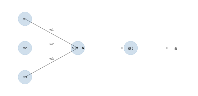
Figure 9.1: a neuron: a weighted sum followed by an activation
9.1.2 The limits of a single neuron
Since a neuron is a linear model followed by a monotone function, its decision boundary is a hyperplane, and it inherits the limitation we already met with the linear discriminant analysis. The classical illustration is the exclusive or, a problem with two binary inputs whose answer is true when exactly one of the two is true.
In R:
xor_df <- data.frame(
  x1 = c(0, 0, 1, 1), x2 = c(0, 1, 0, 1),
  y  = factor(c(0, 1, 1, 0)))

# a logistic regression, that is a single neuron
single <- glm(y ~ x1 + x2, data = xor_df, family = binomial)

gr <- expand.grid(x1 = seq(-.4, 1.4, length.out = 200),
                  x2 = seq(-.4, 1.4, length.out = 200))
gr$p <- predict(single, newdata = gr, type = "response")

x1p <- ggplot(xor_df, aes(x1, x2, colour = y, shape = y)) +
  geom_point(size = 6) + coord_equal() +
  labs(title = "the four points", subtitle = "no line separates the two colours") +
  theme_minimal() + theme(legend.position = "none")

x2p <- ggplot() +
  geom_raster(data = gr, aes(x1, x2, fill = p > .5), alpha = .3) +
  geom_point(data = xor_df, aes(x1, x2, colour = y, shape = y), size = 6) +
  coord_equal() +
  labs(title = "what a single neuron produces",
       subtitle = "it predicts the same class everywhere") +
  theme_minimal() + theme(legend.position = "none")

x1p + x2p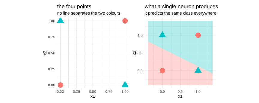
Figure 9.2: the XOR problem cannot be separated by a line
The single neuron is defeated, and not by chance: no straight line can put the two diagonals in different half planes. This failure, pointed out in 1969, stopped research on these models for fifteen years. The solution was already known in principle, and it consists in adding a layer.
9.1.3 The multilayer perceptron
A multilayer perceptron stacks several layers of neurons. Each layer takes the outputs of the previous one as inputs:
\[\begin{align} h^{(1)}&=g\big(W^{(1)}x+b^{(1)}\big) \\ h^{(2)}&=g\big(W^{(2)}h^{(1)}+b^{(2)}\big) \\ &... \\ \hat y&=g_{out}\big(W^{(L)}h^{(L-1)}+b^{(L)}\big) \tag{9.2} \end{align}\]
The layers between the input and the output are called hidden, because nothing in the data says what they should contain: they are the representation the network builds for itself.
The essential point, and the one that deserves to be seen rather than asserted, is why this solves the XOR. The hidden layer applies a transformation to the plane, and in the transformed space the four points become linearly separable. The last layer then only has to draw a line, which it can do. Let us write this network by hand, with two hidden neurons, and look at both spaces.
In R:
set.seed(1)

Xx <- as.matrix(xor_df[, c("x1", "x2")])
yy <- as.numeric(as.character(xor_df$y))

sig  <- function(z) 1 / (1 + exp(-z))
dsig <- function(a) a * (1 - a)

# 2 inputs -> 2 hidden -> 1 output, all written explicitly
W1 <- matrix(rnorm(4, sd = 1.5), 2, 2); b1 <- rnorm(2, sd = .5)
W2 <- matrix(rnorm(2, sd = 1.5), 1, 2); b2 <- rnorm(1, sd = .5)

for (it in 1:20000) {
  H  <- sig(Xx %*% t(W1) + matrix(b1, nrow(Xx), 2, byrow = TRUE))   # hidden
  O  <- sig(H  %*% t(W2) + b2)                                      # output
  dO <- (O - yy) * dsig(O)
  dH <- (dO %*% W2) * dsig(H)
  W2 <- W2 - .5 * t(dO) %*% H ; b2 <- b2 - .5 * sum(dO)
  W1 <- W1 - .5 * t(dH) %*% Xx; b1 <- b1 - .5 * colSums(dH)
}

cat("predictions:", round(as.numeric(O), 3), "\n")
#> predictions: 0.017 0.985 0.985 0.017#> targets : 0 1 1 0hid <- data.frame(h1 = H[, 1], h2 = H[, 2], y = xor_df$y)
o1 <- ggplot(xor_df, aes(x1, x2, colour = y, shape = y)) +
geom_point(size = 6) + coord_equal() +
labs(title = "original space", subtitle = "not separable") +
theme_minimal() + theme(legend.position = "none")
o2 <- ggplot(hid, aes(h1, h2, colour = y, shape = y)) +
geom_point(size = 6) +
geom_abline(intercept = .9, slope = -1, colour = "firebrick", linetype = 2) +
labs(title = "space built by the hidden layer",
subtitle = "a line is now enough") +
theme_minimal() + theme(legend.position = "none")
o1 + o2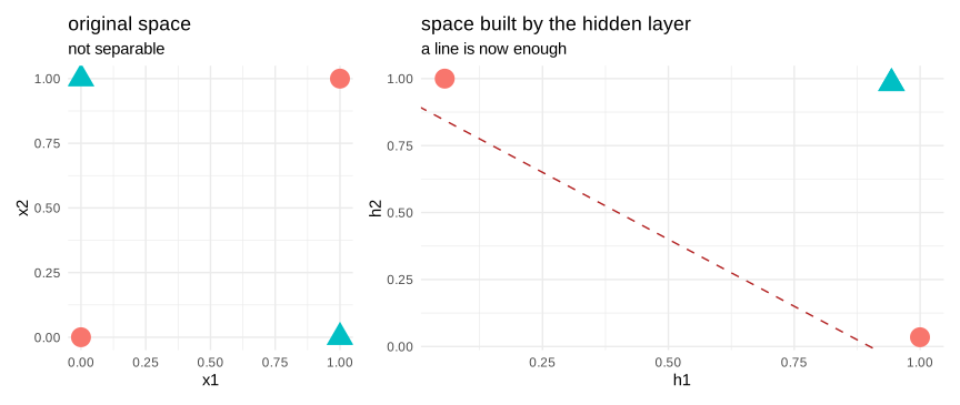
Figure 9.3: the hidden layer makes the problem linearly separable
On the left the two classes are interleaved. On the right, after passing through the two hidden neurons, they occupy two clearly distinct regions and the dashed line separates them. The network did not learn a complicated boundary in the original space; it learned a change of coordinates in which the boundary becomes simple. This is the central idea of the whole chapter, and every architecture that follows is a variation on it.
9.1.4 The universal approximation theorem
How far does this go? The answer is a theorem, proved by Cybenko and by Hornik at the end of the eighties: a network with one hidden layer, containing enough neurons and a non-polynomial activation, can approximate any continuous function on a bounded domain as closely as we wish.
The statement is reassuring and, taken alone, misleading. It says that a solution exists, it does not say that we can find it, nor how many neurons would be needed, and “enough” may mean an astronomical number. Above all, it does not justify depth, since one layer suffices in theory.
What justifies depth is practical. For many functions, a deep network needs exponentially fewer neurons than a shallow one to reach the same accuracy, because it can reuse the intermediate features instead of rebuilding them. A shallow network learns a very wide dictionary; a deep one learns a hierarchy.
The following experiment shows the first half of the theorem at work: as the hidden layer grows, the approximation improves.
In R:
set.seed(123)
f_target <- function(x) sin(3 * x) + 0.4 * cos(7 * x)
xs <- seq(-2, 2, length.out = 200)
ys <- f_target(xs)

fit_mlp <- function(nh, steps = 6000, eta = .02) {
  X1 <- matrix(xs, ncol = 1)
  W1 <- matrix(rnorm(nh, sd = 1), nh, 1); b1 <- rnorm(nh, sd = 1)
  W2 <- matrix(rnorm(nh, sd = .3), 1, nh); b2 <- 0
  for (s in 1:steps) {
    Z1 <- X1 %*% t(W1) + matrix(b1, length(xs), nh, byrow = TRUE)
    H  <- tanh(Z1)
    O  <- as.numeric(H %*% t(W2) + b2)
    dO <- (O - ys) / length(xs)
    dH <- outer(dO, as.numeric(W2)) * (1 - H^2)
    W2 <- W2 - eta * matrix(dO %*% H, 1, nh); b2 <- b2 - eta * sum(dO)
    W1 <- W1 - eta * matrix(colSums(dH * matrix(xs, length(xs), nh)), nh, 1)
    b1 <- b1 - eta * colSums(dH)
  }
  O
}

appro <- do.call(rbind, lapply(c(2, 5, 30), function(nh)
  data.frame(x = xs, truth = ys, fit = fit_mlp(nh),
             lab = paste(nh, "hidden neurons"))))
appro$lab <- factor(appro$lab, levels = unique(appro$lab))

ggplot(appro, aes(x)) +
  geom_line(aes(y = truth), colour = "grey60", linewidth = 1) +
  geom_line(aes(y = fit), colour = "firebrick", linewidth = .8) +
  facet_wrap(~ lab, nrow = 1) +
  labs(title = "the grey curve is the target, the red one the network", y = "") +
  theme_minimal()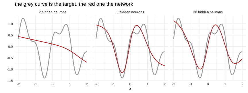
Figure 9.4: a single hidden layer approximates an arbitrary function
With two neurons the network can only produce a coarse shape. With five it follows the main oscillation. With thirty it is almost superimposed on the target. Nothing was changed except the width of the hidden layer.