9.3 Training a network
We now know what a network computes. The question of this section is how its weights are found, and it is the part where nearly all the practical difficulties of deep learning live. A badly trained good architecture performs worse than a well trained modest one.
The principle is the one of the empirical risk minimization introduced in the previous chapter: choose the parameters that minimize the average loss on the training set. What is new is that the function to minimize is no longer convex, that it depends on millions of parameters, and that its gradient must be obtained without ever writing it down by hand.
9.3.1 Forward propagation
The forward pass is the evaluation of the network on an input. For a network with two hidden layers it is the chain:
\[\begin{align} z^{(1)}&=W^{(1)}x+b^{(1)} \quad &a^{(1)}&=g(z^{(1)}) \\ z^{(2)}&=W^{(2)}a^{(1)}+b^{(2)} \quad &a^{(2)}&=g(z^{(2)}) \\ z^{(3)}&=W^{(3)}a^{(2)}+b^{(3)} \quad &\hat y&=g_{out}(z^{(3)}) \tag{9.7} \end{align}\]
Two quantities are distinguished at every layer, and the distinction matters for what follows: the pre-activation \(z\), which is linear in the inputs of the layer, and the activation \(a=g(z)\). The pre-activations must be kept in memory during the forward pass, because the backward pass will need them. This is the reason why training a network consumes far more memory than using one.
In practice the observations are processed by blocks. If \(X\) is a matrix with one observation per row, the whole layer is a single matrix product, which is what makes these models fast on the hardware designed for that operation.
9.3.2 The loss function
The loss is chosen according to the output, exactly as in the previous chapter:
\[\begin{align} \text{regression}&: \quad L=\frac{1}{n}\sum_{i=1}^{n}(y_i-\hat y_i)^2 \\ \text{binary}&: \quad L=-\frac{1}{n}\sum_{i=1}^{n}\Big(y_i\ln\hat y_i+(1-y_i)\ln(1-\hat y_i)\Big) \\ \text{multi-class}&: \quad L=-\frac{1}{n}\sum_{i=1}^{n}\sum_{k=1}^{K}y_{ik}\ln\hat y_{ik} \tag{9.8} \end{align}\]
The pairing of the last activation with the loss is not arbitrary. When the sigmoid is combined with the log loss, or the softmax with the cross entropy, an algebraic simplification occurs that we will meet in a moment: the gradient at the output reduces to \(\hat y-y\), the error itself. The derivative of the activation, which could have been small, disappears from the expression. Pairing a sigmoid with a quadratic loss instead keeps that factor and produces a network that learns very slowly precisely when it is very wrong, which is the opposite of what we want.
9.3.3 Backpropagation
Backpropagation is nothing more than the chain rule, applied in the right order. It is worth deriving once, because everything that follows, including the vanishing gradient problem, is read directly off the formulas.
We want \(\frac{\partial L}{\partial W^{(l)}}\) for every layer. Define the error of a layer as the derivative of the loss with respect to its pre-activation:
\[\begin{equation} \delta^{(l)}=\frac{\partial L}{\partial z^{(l)}} \tag{9.9} \end{equation}\]
At the last layer, with the pairing mentioned above:
\[\begin{equation} \delta^{(L)}=\hat y-y \tag{9.10} \end{equation}\]
Then, for any earlier layer, the chain rule gives the recurrence that gives the method its name:
\[\begin{equation} \delta^{(l)}=\Big(W^{(l+1)t}\delta^{(l+1)}\Big)\odot g'(z^{(l)}) \tag{9.11} \end{equation}\]
where \(\odot\) is the element by element product. The error of a layer is the error of the next one, pushed back through the weights, and multiplied by the derivative of the activation. Once the \(\delta\) are known, the gradients are immediate:
\[\begin{align} \frac{\partial L}{\partial W^{(l)}}&=\delta^{(l)}a^{(l-1)t} \\ \frac{\partial L}{\partial b^{(l)}}&=\delta^{(l)} \tag{9.12} \end{align}\]
Equation (9.11) deserves to be looked at, because it contains the whole story of the next sections. Going down one layer multiplies the error by a weight matrix and by the derivative of the activation. If those factors are smaller than one, the gradient shrinks at every layer; if they are larger, it grows.
Let us implement this on a real problem, and above all verify it. A derivation can always contain a sign error, and there is a simple way to check: compare the analytic gradient with a numerical one obtained by perturbing each parameter.
In R:
set.seed(123)

# a small two class problem in two dimensions
n <- 400
Xn <- matrix(rnorm(n * 2), n, 2)
yn <- as.numeric(Xn[, 1]^2 + Xn[, 2]^2 > 1.6)   # a circular frontier

relu  <- function(z) pmax(z, 0)
drelu <- function(z) as.numeric(z > 0)
sigm  <- function(z) 1 / (1 + exp(-z))

init_net <- function(p, h, seed = 1) {
  set.seed(seed)
  list(W1 = matrix(rnorm(h * p, sd = sqrt(2 / p)), h, p), b1 = rep(0, h),
       W2 = matrix(rnorm(h,     sd = sqrt(2 / h)), 1, h), b2 = 0)
}

forward <- function(net, X) {
  Z1 <- X %*% t(net$W1) + matrix(net$b1, nrow(X), length(net$b1), byrow = TRUE)
  A1 <- relu(Z1)
  Z2 <- as.numeric(A1 %*% t(net$W2) + net$b2)
  list(Z1 = Z1, A1 = A1, Z2 = Z2, yhat = sigm(Z2))
}

loss_fn <- function(yhat, y) {
  eps <- 1e-9
  -mean(y * log(yhat + eps) + (1 - y) * log(1 - yhat + eps))
}

backward <- function(net, X, y, fw) {
  m <- nrow(X)
  d2 <- (fw$yhat - y) / m                      # delta of the output layer
  gW2 <- matrix(d2 %*% fw$A1, 1, ncol(fw$A1))
  gb2 <- sum(d2)
  d1 <- outer(d2, as.numeric(net$W2)) * drelu(fw$Z1)   # the recurrence
  gW1 <- t(d1) %*% X
  gb1 <- colSums(d1)
  list(W1 = gW1, b1 = gb1, W2 = gW2, b2 = gb2)
}

net <- init_net(2, 8)
fw  <- forward(net, Xn)
gr  <- backward(net, Xn, yn, fw)
The gradient check compares each analytic derivative with \(\frac{L(\theta+\epsilon)-L(\theta-\epsilon)}{2\epsilon}\).
num_grad <- function(net, X, y, name, i, j = NULL, eps = 1e-5) {
  bump <- function(s) {
    n2 <- net
    if (is.null(j)) n2[[name]][i] <- n2[[name]][i] + s
    else            n2[[name]][i, j] <- n2[[name]][i, j] + s
    loss_fn(forward(n2, X)$yhat, y)
  }
  (bump(eps) - bump(-eps)) / (2 * eps)
}

check <- data.frame(
  parameter = c("W1[1,1]", "W1[3,2]", "b1[2]", "W2[1,4]", "b2"),
  analytic = c(gr$W1[1, 1], gr$W1[3, 2], gr$b1[2], gr$W2[1, 4], gr$b2),
  numeric  = c(num_grad(net, Xn, yn, "W1", 1, 1),
               num_grad(net, Xn, yn, "W1", 3, 2),
               num_grad(net, Xn, yn, "b1", 2),
               num_grad(net, Xn, yn, "W2", 1, 4),
               num_grad(net, Xn, yn, "b2", 1)))
check$abs_difference <- abs(check$analytic - check$numeric)| parameter | analytic | numeric | abs_difference |
|---|---|---|---|
| W1[1,1] | 0.0002700105 | 0.0002700105 | 0e+00 |
| W1[3,2] | 0.0157562580 | 0.0157562579 | 1e-10 |
| b1[2] | 0.0483952371 | 0.0483952370 | 2e-10 |
| W2[1,4] | -0.0494579804 | -0.0494579804 | 0e+00 |
| b2 | 0.2377062059 | 0.2377062051 | 8e-10 |
The differences are of the order of the precision of the numerical approximation, which confirms that the derivation is correct. This check costs a few lines and should be performed every time a gradient is written by hand; it is the only way to distinguish a genuine bug from a network that simply learns badly.
We can now train the network and watch it learn the circular boundary.
train <- function(net, X, y, eta = .5, steps = 4000) {
  hist <- numeric(steps)
  for (s in 1:steps) {
    fw <- forward(net, X)
    hist[s] <- loss_fn(fw$yhat, y)
    g  <- backward(net, X, y, fw)
    net$W1 <- net$W1 - eta * g$W1; net$b1 <- net$b1 - eta * g$b1
    net$W2 <- net$W2 - eta * g$W2; net$b2 <- net$b2 - eta * g$b2
  }
  list(net = net, hist = hist)
}

res <- train(init_net(2, 8), Xn, yn)

gx <- seq(-3, 3, length.out = 160)
grid_dl <- as.matrix(expand.grid(x1 = gx, x2 = gx))
pgrid <- forward(res$net, grid_dl)$yhat
gdf <- data.frame(grid_dl, p = pgrid)

t1 <- ggplot(data.frame(step = seq_along(res$hist), loss = res$hist),
             aes(step, loss)) +
  geom_line(colour = "firebrick") +
  labs(title = "the loss during training") + theme_minimal()

t2 <- ggplot() +
  geom_raster(data = gdf, aes(x1, x2, fill = p), alpha = .7) +
  scale_fill_gradient2(low = "white", mid = "grey90", high = "steelblue",
                       midpoint = .5) +
  geom_point(data = data.frame(Xn, y = factor(yn)),
             aes(X1, X2, colour = y), size = .8) +
  coord_equal() + labs(title = "the boundary found") +
  theme_minimal() + theme(legend.position = "none")

t1 + t2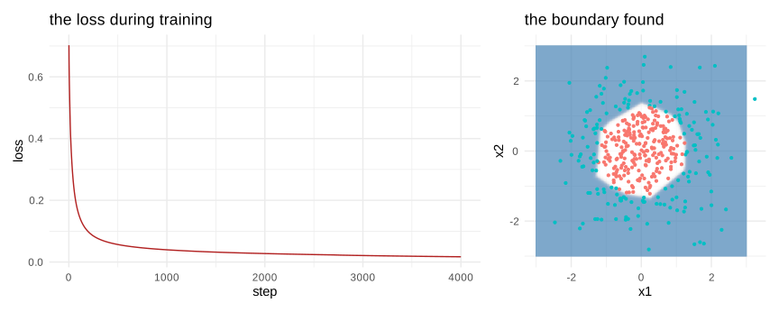
Figure 9.8: the network learns a boundary that a linear model cannot
9.3.4 Gradient descent and its variants
The update used above is the plain gradient descent, \(\theta \leftarrow \theta-\eta\,\nabla L\). It has a weakness that becomes severe in high dimension: when the loss surface is a narrow valley, steep in one direction and nearly flat in another, the gradient points mostly across the valley rather than along it, and the trajectory oscillates from one wall to the other while advancing slowly.
Four ideas, each building on the previous one, fix this.
Momentum accumulates the past gradients in a velocity, exactly as a heavy ball would keep its direction:
\[\begin{align} v&\leftarrow \beta v+(1-\beta)\nabla L \\ \theta&\leftarrow \theta-\eta v \tag{9.13} \end{align}\]
The oscillating components cancel each other between successive steps while the consistent direction adds up, so the ball rolls along the valley instead of bouncing.
RMSProp attacks the other half of the problem, the fact that a single learning rate must serve parameters with very different scales. It keeps a running average of the squared gradients and divides by its root:
\[\begin{align} s&\leftarrow \rho s+(1-\rho)(\nabla L)^2 \\ \theta&\leftarrow \theta-\frac{\eta}{\sqrt{s}+\epsilon}\nabla L \tag{9.14} \end{align}\]
Each parameter thus receives its own effective rate, large where the gradient has been small and small where it has been large.
Adam combines the two, with a bias correction for the first iterations, and is the default choice in practice:
\[\begin{align} v&\leftarrow \beta_1 v+(1-\beta_1)\nabla L, \qquad \hat v=\frac{v}{1-\beta_1^t} \\ s&\leftarrow \beta_2 s+(1-\beta_2)(\nabla L)^2, \qquad \hat s=\frac{s}{1-\beta_2^t} \\ \theta&\leftarrow \theta-\frac{\eta}{\sqrt{\hat s}+\epsilon}\hat v \tag{9.15} \end{align}\]
The recommended values, \(\beta_1=0.9\) and \(\beta_2=0.999\), work so often that they are rarely changed.
In R:
# an elongated quadratic bowl: gentle along x, steep along y
f_surf  <- function(p) 0.06 * p[1]^2 + 2.2 * p[2]^2
g_surf  <- function(p) c(0.12 * p[1], 4.4 * p[2])

run_opt <- function(kind, steps = 90, eta = .12) {
  p <- c(-9, 2.2); v <- c(0, 0); s <- c(0, 0); path <- p
  for (t in 1:steps) {
    g <- g_surf(p)
    if (kind == "gradient descent")      p <- p - eta * g
    if (kind == "momentum") { v <- .9 * v + .1 * g;  p <- p - eta * 10 * v }
    if (kind == "RMSProp")  { s <- .9 * s + .1 * g^2; p <- p - eta * g / (sqrt(s) + 1e-8) }
    if (kind == "Adam") {
      v <- .9 * v + .1 * g; s <- .999 * s + .001 * g^2
      vh <- v / (1 - .9^t); sh <- s / (1 - .999^t)
      p <- p - eta * 3 * vh / (sqrt(sh) + 1e-8)
    }
    path <- rbind(path, p)
  }
  data.frame(x = path[, 1], y = path[, 2], opt = kind, step = 0:steps)
}

paths <- do.call(rbind, lapply(
  c("gradient descent", "momentum", "RMSProp", "Adam"), run_opt))

srf <- expand.grid(x = seq(-10, 10, length.out = 160),
                   y = seq(-3, 3, length.out = 160))
srf$z <- 0.06 * srf$x^2 + 2.2 * srf$y^2

ggplot() +
  geom_contour(data = srf, aes(x, y, z = z), bins = 22,
               colour = "grey80", linewidth = .3) +
  geom_path(data = paths, aes(x, y, colour = opt), linewidth = .8) +
  # the layer needs its own data frame: a data-less layer cannot be
  # assigned to the panels of a facet
  geom_point(data = data.frame(x = 0, y = 0), aes(x, y),
             colour = "firebrick", shape = 4, size = 3) +
  facet_wrap(~ opt) + coord_equal() +
  labs(title = "the same surface, the same starting point, four rules",
       subtitle = "the cross marks the minimum") +
  theme_minimal() + theme(legend.position = "none")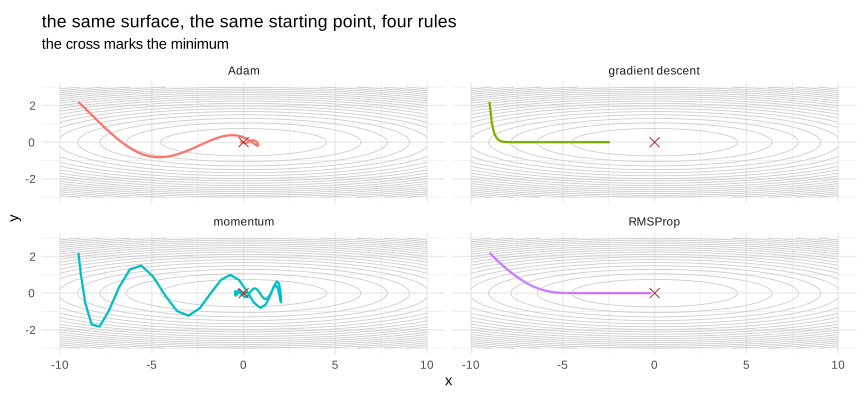
Figure 9.9: four optimizers in a narrow valley
The four trajectories start at the same place. Plain gradient descent zigzags across the valley and crawls towards the minimum. Momentum damps the oscillation and travels much further along the flat direction. RMSProp rescales the two axes and goes almost straight. Adam, combining both, reaches the neighbourhood of the minimum first.
9.3.5 The learning rate
The learning rate is the single most important hyperparameter of a network, and it is worth spending time on it before anything else. Its effect is best understood from a picture rather than a rule.
In R:
lr_run <- function(eta, steps = 60) {
  p <- c(-9, 2.2); path <- p
  for (t in 1:steps) { p <- p - eta * g_surf(p); path <- rbind(path, p) }
  data.frame(x = path[, 1], y = path[, 2],
             lab = paste("eta =", eta), step = 0:steps)
}

lr_paths <- rbind(lr_run(0.02), lr_run(0.22), lr_run(0.47))
lr_paths$lab <- factor(lr_paths$lab, levels = unique(lr_paths$lab))
lr_paths <- subset(lr_paths, abs(x) < 12 & abs(y) < 3.2)

ggplot() +
  geom_contour(data = srf, aes(x, y, z = z), bins = 22,
               colour = "grey80", linewidth = .3) +
  geom_path(data = lr_paths, aes(x, y), colour = "firebrick", linewidth = .7) +
  geom_point(data = lr_paths, aes(x, y), colour = "firebrick", size = .5) +
  facet_wrap(~ lab) + coord_equal(xlim = c(-10, 10), ylim = c(-3, 3)) +
  labs(title = "too small, about right, too large") +
  theme_minimal()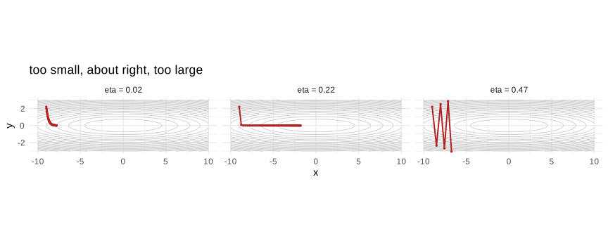
Figure 9.10: three learning rates on the same problem
On the left the steps are tiny and the trajectory has barely moved after sixty iterations: the training would eventually succeed, but at a cost nobody would pay. In the middle it advances steadily. On the right the steps overshoot the valley and the trajectory bounces between the walls, growing instead of shrinking, and the loss diverges.
The practical signature of each case is visible on the loss curve: a flat, slowly decreasing line means the rate is too small; a curve that decreases then explodes, or that returns NaN, means it is too large. The usual method is to try a geometric grid, \(10^{-1},10^{-2},10^{-3},10^{-4}\), and keep the largest value that still decreases cleanly.
It is also common to decrease the rate during training, since large steps are useful at the beginning and harmful near the minimum. The usual schedules divide it by a constant every so many epochs, or follow a cosine curve towards zero.
9.3.6 Batch, epoch and mini-batch
Three words are constantly used and easily confused:
a batch is the group of observations used to compute one gradient and perform one update;
an iteration is one such update;
an epoch is one complete pass through the training set, and therefore contains \(n/\text{batch size}\) iterations.
The choice of the batch size is a compromise between two extremes. Taking the whole sample gives the exact gradient and a smooth trajectory, but one update per epoch and a prohibitive memory cost. Taking a single observation, which is the stochastic descent of the previous chapter, gives very cheap and very noisy updates. Mini-batches of a few tens to a few hundreds sit in between and are what everyone uses, also because a matrix product on a block is far more efficient on the hardware than many small ones.
The noise introduced by small batches is not only a defect. It acts as a mild regularizer and helps the trajectory escape from the poor regions of a non-convex surface, which is one reason why very large batches sometimes generalize slightly worse.
set.seed(1)
train_mb <- function(bs, epochs = 40, eta = .5) {
  net <- init_net(2, 8); hist <- c()
  for (e in 1:epochs) {
    idx <- sample(nrow(Xn))
    for (start in seq(1, nrow(Xn), by = bs)) {
      take <- idx[start:min(start + bs - 1, nrow(Xn))]
      fw <- forward(net, Xn[take, , drop = FALSE])
      g  <- backward(net, Xn[take, , drop = FALSE], yn[take], fw)
      net$W1 <- net$W1 - eta * g$W1; net$b1 <- net$b1 - eta * g$b1
      net$W2 <- net$W2 - eta * g$W2; net$b2 <- net$b2 - eta * g$b2
    }
    hist <- c(hist, loss_fn(forward(net, Xn)$yhat, yn))
  }
  data.frame(epoch = seq_along(hist), loss = hist,
             lab = paste("batch =", bs))
}

mb <- rbind(train_mb(8), train_mb(64), train_mb(400))
mb$lab <- factor(mb$lab, levels = unique(mb$lab))

ggplot(mb, aes(epoch, loss, colour = lab)) +
  geom_line(linewidth = .8) +
  labs(title = "loss per epoch for three batch sizes",
       subtitle = "small batches make more updates per epoch, and a noisier curve") +
  theme_minimal()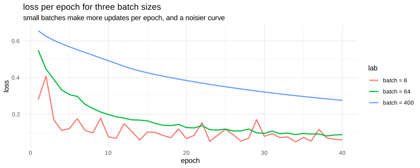
Figure 9.11: the size of the batch changes the shape of the trajectory
For an equal number of epochs, the small batch has performed fifty times more updates than the full batch and has therefore progressed much further, at the price of a visibly noisier curve. This is the usual trade, and it explains why the batch size is almost always chosen small relative to the sample.
9.3.7 Vanishing and exploding gradients
We can now return to equation (9.11) and read the consequence that blocked the field for two decades. Going back through \(L\) layers multiplies the error by \(L\) weight matrices and by \(L\) derivatives of the activation. The magnitude of the gradient at the first layer is therefore governed by a product of many factors.
If those factors are on average smaller than one, the product tends to zero exponentially with depth: the first layers receive almost no signal and stop learning. This is the vanishing gradient. If they are larger than one, the product explodes, the updates become enormous and the loss returns NaN. This is the exploding gradient.
The sigmoid guarantees the first case, since its derivative never exceeds \(0.25\): ten layers multiply the gradient by at most \(0.25^{10}\approx 10^{-6}\). The measurement below makes the phenomenon concrete.
In R:
set.seed(1)

grad_profile <- function(activation, L = 12, width = 24) {
  g  <- switch(activation,
               sigmoid = function(z) 1 / (1 + exp(-z)),
               relu    = function(z) pmax(z, 0))
  gp <- switch(activation,
               sigmoid = function(z) { s <- 1 / (1 + exp(-z)); s * (1 - s) },
               relu    = function(z) as.numeric(z > 0))

  x <- matrix(rnorm(width), 1, width)
  Ws <- lapply(1:L, function(i) matrix(rnorm(width * width, sd = .5), width, width))
  Zs <- vector("list", L); A <- x
  for (l in 1:L) { Zs[[l]] <- A %*% Ws[[l]]; A <- g(Zs[[l]]) }

  delta <- matrix(rnorm(width), 1, width)      # an arbitrary error at the output
  norms <- numeric(L)
  for (l in L:1) {
    delta <- delta * gp(Zs[[l]])
    norms[l] <- sqrt(sum(delta^2))
    delta <- delta %*% t(Ws[[l]])
  }
  data.frame(layer = 1:L, norm = norms, activation = activation)
}

prof <- rbind(grad_profile("sigmoid"), grad_profile("relu"))

ggplot(prof, aes(layer, norm, colour = activation)) +
  geom_line(linewidth = .9) + geom_point() +
  scale_y_log10() +
  labs(title = "norm of the gradient at each layer, on a log scale",
       subtitle = "layer 1 is the input side, layer 12 the output side",
       y = "gradient norm (log)") +
  theme_minimal()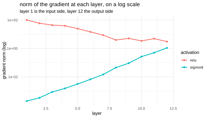
Figure 9.12: the gradient across the layers of a deep network
The vertical scale is logarithmic, and a straight line on it is an exponential decay. With the sigmoid the gradient loses several orders of magnitude between the output and the input, so the early layers are effectively frozen. With the ReLU the profile is far flatter.
Four remedies are used, and we have already met or will meet all of them: the ReLU family, which keeps a derivative of one; a careful initialization, treated next; batch normalization, which rescales the pre-activations at every layer; and the residual connections, which add a shortcut \(a^{(l+1)}=a^{(l)}+f(a^{(l)})\) so that the gradient has a path of multiplier one back to the early layers. That last idea is what made networks of hundreds of layers trainable.
For the exploding case the standard remedy is simpler still: gradient clipping, which rescales the gradient whenever its norm exceeds a threshold.
9.3.8 The initialization of the weights
The starting point matters, and for a reason that follows the same arithmetic. Two naive choices fail immediately.
Initializing every weight to zero makes all the neurons of a layer compute the same thing, receive the same gradient and stay identical forever: the layer behaves like a single neuron. This is the symmetry problem, and it is why the initialization must be random.
Initializing with a variance that is too large or too small makes the activations grow or shrink at every layer, and the gradient with them. The sensible rule is to choose the variance so that the signal keeps roughly the same magnitude from one layer to the next, which gives:
\[\begin{align} \text{Xavier (for tanh)}&: \quad Var(w)=\frac{2}{n_{in}+n_{out}} \\ \text{He (for ReLU)}&: \quad Var(w)=\frac{2}{n_{in}} \tag{9.16} \end{align}\]
The He variant carries a factor two because the ReLU sets half of its inputs to zero and therefore halves the variance of the output.
In R:
set.seed(1)
prop_act <- function(sd_w, label, L = 8, width = 200) {
  A <- matrix(rnorm(width), 1, width)
  out <- data.frame()
  for (l in 1:L) {
    W <- matrix(rnorm(width * width, sd = sd_w), width, width)
    A <- pmax(A %*% W, 0)
    out <- rbind(out, data.frame(layer = l, sd = sd(as.numeric(A)), kind = label))
  }
  out
}

w <- 200
ini <- rbind(
  prop_act(0.02,             "too small"),
  prop_act(sqrt(2 / w),      "He (2/n_in)"),
  prop_act(0.2,              "too large"))

ggplot(ini, aes(layer, sd, colour = kind)) +
  geom_line(linewidth = .9) + geom_point() +
  scale_y_log10() +
  labs(title = "standard deviation of the activations, layer by layer",
       y = "sd (log scale)") +
  theme_minimal()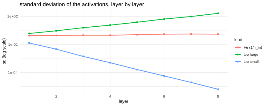
Figure 9.13: the distribution of the activations through the layers
With a variance that is too small the signal dies out after a few layers and nothing reaches the output. With a variance that is too large it grows until it saturates the arithmetic. The He initialization keeps it almost constant, which is exactly what it was designed for. The same three curves would be obtained for the gradient on the way back, which is why this choice matters so much.
In Python:
Everything written by hand above is available in one line in a framework. We use PyTorch, whose automatic differentiation computes the backward pass for any expression we write.
#> <torch._C.Generator object at 0x0000020E2AABD510>
Xt = torch.tensor(np.asarray(Xn_py), dtype=torch.float32)
yt = torch.tensor(np.asarray(yn_py), dtype=torch.float32).view(-1, 1)

model = nn.Sequential(
    nn.Linear(2, 8),
    nn.ReLU(),
    nn.Linear(8, 1),
)
loss_fn_t = nn.BCEWithLogitsLoss()          # sigmoid and log loss combined
opt = torch.optim.Adam(model.parameters(), lr=0.05)

hist = []
for step in range(1500):
    opt.zero_grad()
    out = model(Xt)
    loss = loss_fn_t(out, yt)
    loss.backward()                          # the whole backward pass
    opt.step()
    hist.append(loss.item())

acc = ((torch.sigmoid(model(Xt)) > .5).float() == yt).float().mean().item()
torch_tab = pd.DataFrame({"final_loss": [round(hist[-1], 4)],
                          "accuracy": [round(acc, 4)],
"parameters": [sum(p.numel() for p in model.parameters())]})| final_loss | accuracy | parameters |
|---|---|---|
| 0.0044 | 1 | 33 |
The three lines loss.backward(), opt.step() and opt.zero_grad() replace the whole backward function we wrote above. It is worth remembering what they hide: backward walks the graph of operations in reverse and applies equation (9.11) at every node, step applies the update rule of the chosen optimizer, and zero_grad erases the gradients of the previous iteration, because PyTorch accumulates them by default. Forgetting that last call is the most common beginner’s mistake, and it produces a network that seems to train and does not.
#> <Figure size 600x300 with 0 Axes>#> [<matplotlib.lines.Line2D object at 0x0000020F2C690920>]#> Text(0.5, 0, 'iteration')
#> Text(0, 0.5, 'loss')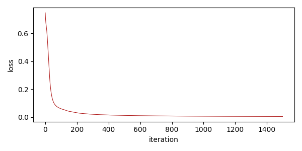
Figure 9.14: training a network with PyTorch