7.4 ARCH AND GARCH MODELS
All the models of the previous section describe the mean of the series and treat the variance of the errors as a constant, \(Var(\varepsilon_t)=\sigma^2\). This assumption is comfortable, but it is contradicted by most financial series. When we look at the returns of an exchange rate or of a stock index, we observe that calm periods and agitated periods follow each other: a large variation is usually followed by another large variation, of either sign, and a small one by another small one. This phenomenon is called volatility clustering, and it means that the variance of the error is not constant but depends on the past.
The important point is that this is not the heteroskedasticity we met in the chapter on the assumptions on the disturbances. There the variance depended on the explanatory variables, and the remedy was to correct the standard errors. Here the variance depends on its own past, it is conditional on the information available at the date \(t-1\), and it is an object that we want to model for itself, because in finance the volatility is exactly what we try to forecast.
We therefore write the series as a mean part plus an error whose conditional variance evolves over time:
\[\begin{equation} \varepsilon_t=\sigma_t z_t \quad \text{with} \quad z_t \sim iid(0,1) \tag{7.39} \end{equation}\]
where \(z_t\) is a standardized white noise and \(\sigma_t\) is the conditional standard deviation. The models of this section differ only in the way they specify \(\sigma_t^2\).
To illustrate them, we simulate a series that has this property by construction.
In R:
set.seed(123)

n <- 1500
omega <- 0.05; alpha <- 0.10; beta <- 0.85

eps  <- numeric(n)
sig2 <- numeric(n)
sig2[1] <- omega / (1 - alpha - beta)
eps[1]  <- sqrt(sig2[1]) * rnorm(1)

for (t in 2:n) {
  sig2[t] <- omega + alpha * eps[t - 1]^2 + beta * sig2[t - 1]
  eps[t]  <- sqrt(sig2[t]) * rnorm(1)
}

garch_ts <- ts(eps)
plot(garch_ts, main = "simulated returns", ylab = "")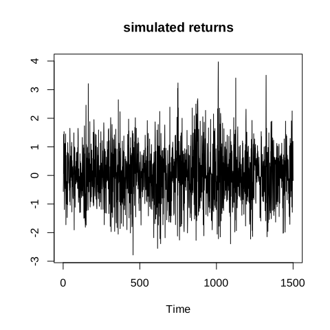
Figure 7.26: a simulated series with volatility clustering
The series oscillates around zero, as a white noise would, but the amplitude of the oscillations is visibly not constant. Periods of strong movements alternate with quiet ones, which is what we wanted to reproduce.
A useful remark is that the series itself is not autocorrelated, while its square is. This is the practical signature of conditional heteroskedasticity, and it is the first thing to look at.
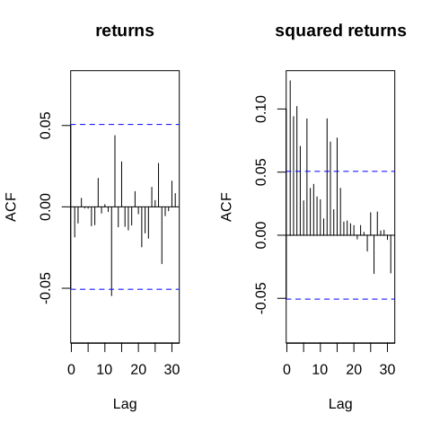
Figure 7.27: correlogram of the series and of its square
The correlogram of the returns shows almost nothing, so an \(ARIMA\) model would conclude that the series is a white noise and stop there. The correlogram of the squared returns, on the contrary, is full of significant spikes, which proves that the series is not independent: it is only uncorrelated.
7.4.1 ARCH model
Engle proposed in 1982 to make the conditional variance an auto-regressive function of the past squared errors. The \(ARCH(q)\) model, for autoregressive conditional heteroskedasticity, is written:
\[\begin{equation} \sigma_t^2=\alpha_0+\alpha_1\varepsilon_{t-1}^2+...+\alpha_q\varepsilon_{t-q}^2 \tag{7.40} \end{equation}\]
The interpretation is direct: a large shock at the date \(t-1\), whatever its sign since it is squared, raises the variance at the date \(t\). For the variance to be positive we impose \(\alpha_0>0\) and \(\alpha_i\geqslant 0\), and for the unconditional variance to exist we need \(\sum\alpha_i<1\), in which case it equals \(\frac{\alpha_0}{1-\sum\alpha_i}\).
Before estimating such a model we test whether it is needed at all. The ARCH-LM test of Engle regresses the squared residuals on their own \(q\) lags and tests the joint nullity of the coefficients:
\[\begin{equation} \varepsilon_t^2=\alpha_0+\alpha_1\varepsilon_{t-1}^2+...+\alpha_q\varepsilon_{t-q}^2+u_t \tag{7.41} \end{equation}\]
Under the null hypothesis of no ARCH effect, the statistic \(nR^2\) follows a \(\chi^2(q)\) distribution.
In R:
The test is short enough to be written directly, which also makes its logic explicit.
# ARCH-LM test written by hand
arch_lm <- function(x, q = 5) {
  e2  <- as.numeric(x)^2
  df  <- embed(e2, q + 1)
  reg <- lm(df[, 1] ~ df[, -1])
  r2  <- summary(reg)$r.squared
  stat <- nrow(df) * r2
  data.frame(statistic = stat, df = q,
             p_value = pchisq(stat, df = q, lower.tail = FALSE))
}

arch_test <- arch_lm(garch_ts, q = 5)| statistic | df | p_value |
|---|---|---|
| 44.9624 | 5 | 0 |
The p-value is essentially zero, so the hypothesis of a constant conditional variance is rejected and an ARCH type model is justified.
We now estimate an \(ARCH(1)\) with the package rugarch, which specifies the model in two parts, the variance equation and the mean equation, and then fits it by maximum likelihood.
suppressPackageStartupMessages(library(rugarch))

arch_spec <- ugarchspec(
  variance.model = list(model = "sGARCH", garchOrder = c(1, 0)),
  mean.model     = list(armaOrder = c(0, 0), include.mean = FALSE)
)
arch_fit <- ugarchfit(arch_spec, data = garch_ts, solver = "hybrid")

arch_out <- data.frame(
  coefficient = names(coef(arch_fit)),
  estimate    = as.numeric(coef(arch_fit))
)| coefficient | estimate |
|---|---|
| omega | 0.7970 |
| alpha1 | 0.1056 |
The coefficient \(\alpha_1\) is significant, but it is far from capturing the whole persistence of the volatility that we built into the simulation. An \(ARCH(1)\) only remembers one period, and reproducing a long memory would require a large \(q\), hence many coefficients. This is precisely the problem that the next model solves.
7.4.2 GARCH model
Bollerslev generalized the previous specification in 1986 by adding to it the lagged conditional variances, exactly as the moving average part was added to the auto-regressive one. The \(GARCH(p,q)\) is written:
\[\begin{equation} \sigma_t^2=\alpha_0+\sum_{i=1}^{q}\alpha_i\varepsilon_{t-i}^2+\sum_{j=1}^{p}\beta_j\sigma_{t-j}^2 \tag{7.42} \end{equation}\]
The term \(\beta_j\sigma_{t-j}^2\) plays the same role of parsimony as the moving average part did for the mean: a \(GARCH(1,1)\) with three coefficients reproduces a persistence that would require an \(ARCH\) of high order. This is why it has become the standard model, and why it is very often sufficient in practice.
Two quantities are read directly on the estimated coefficients. The sum \(\alpha_1+\beta_1\) measures the persistence of the volatility: the closer it is to one, the longer a shock keeps influencing the variance. And the unconditional variance, which exists only if this sum is smaller than one, is given by:
\[\begin{equation} \sigma^2=\frac{\alpha_0}{1-\alpha_1-\beta_1} \tag{7.43} \end{equation}\]
In R:
garch_spec <- ugarchspec(
  variance.model = list(model = "sGARCH", garchOrder = c(1, 1)),
  mean.model     = list(armaOrder = c(0, 0), include.mean = FALSE)
)
garch_fit <- ugarchfit(garch_spec, data = garch_ts, solver = "hybrid")

garch_out <- data.frame(
  coefficient = names(coef(garch_fit)),
  true_value  = c(omega, alpha, beta),
  estimate    = as.numeric(coef(garch_fit))
)| coefficient | true_value | estimate |
|---|---|---|
| omega | 0.05 | 0.0759 |
| alpha1 | 0.10 | 0.0871 |
| beta1 | 0.85 | 0.8285 |
The three estimates are close to the values used in the simulation. The persistence is obtained by adding the last two.
pers <- sum(coef(garch_fit)[c("alpha1", "beta1")])
cat("persistence alpha1 + beta1 =", round(pers, 4), "\n")
#> persistence alpha1 + beta1 = 0.9155#> unconditional variance = 0.8988The persistence is high, above \(0.9\), which is typical of financial series, and it says that a shock on the volatility is absorbed only slowly.
The estimated conditional standard deviation can be plotted along the series, and it follows the periods of agitation.
plot(as.numeric(sigma(garch_fit)), type = "l",
     xlab = "time", ylab = "conditional standard deviation",
     main = "volatility estimated by the GARCH(1,1)")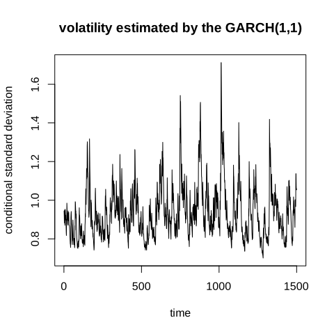
Figure 7.28: estimated conditional volatility in R
In Python:
The package arch provides the same family of models through the function arch_model.
from arch import arch_model

garch_fit_py = arch_model(garch_py, mean="Zero", vol="GARCH", p=1, q=1).fit(disp="off")

garch_out_py = pd.DataFrame({
    "coefficient": list(garch_fit_py.params.index),
    "estimate": [round(v, 4) for v in garch_fit_py.params],
    "std_error": [round(v, 4) for v in garch_fit_py.std_err]
})| coefficient | estimate | std_error |
|---|---|---|
| omega | 0.0760 | 0.0277 |
| alpha[1] | 0.0868 | 0.0227 |
| beta[1] | 0.8286 | 0.0456 |
The names differ, omega, alpha[1] and beta[1] instead of the R ones, but the values are the same.
7.4.3 TGARCH MODEL
The two previous models share a property that the data contradict: the conditional variance depends on \(\varepsilon_{t-1}^2\), so a positive shock and a negative shock of the same magnitude have exactly the same effect on the future volatility. On financial markets this symmetry does not hold. A fall of the prices raises the volatility much more than a rise of the same size, a phenomenon known as the leverage effect, and explained by the fact that a fall increases the debt to equity ratio of the firms and therefore the risk perceived by the investors.
The threshold models break this symmetry by letting the coefficient of the past shock depend on its sign. In the form proposed by Glosten, Jagannathan and Runkle, which is the one implemented identically in both languages, the variance equation becomes:
\[\begin{equation} \sigma_t^2=\alpha_0+\alpha_1\varepsilon_{t-1}^2+\gamma \varepsilon_{t-1}^2 I_{\{\varepsilon_{t-1}<0\}}+\beta_1\sigma_{t-1}^2 \tag{7.44} \end{equation}\]
where \(I_{\{\varepsilon_{t-1}<0\}}\) is an indicator that equals one when the previous shock was negative and zero otherwise. A positive shock therefore has the effect \(\alpha_1\), while a negative shock has the effect \(\alpha_1+\gamma\). The leverage effect corresponds to \(\gamma>0\), and testing its significance is the same as testing the symmetry of the reaction.
The literature uses several close names for these models. The specification above is usually called GJR-GARCH, while the TGARCH of Zakoian writes the same idea on the conditional standard deviation instead of the variance. The two lead to the same conclusions on the asymmetry, and we use here the GJR form because R and python implement it in exactly the same way.
Our simulated series was generated by a symmetric \(GARCH\), so we expect \(\gamma\) to be small and not significant. To make the illustration meaningful, we build a second series that does contain a leverage effect.
In R:
set.seed(123)

# simulation of a series with a leverage effect: gamma = 0.15
gam <- 0.15
eps_a  <- numeric(n)
sig2_a <- numeric(n)
sig2_a[1] <- omega / (1 - alpha - beta)
eps_a[1]  <- sqrt(sig2_a[1]) * rnorm(1)

for (t in 2:n) {
  neg <- as.numeric(eps_a[t - 1] < 0)
  sig2_a[t] <- omega + (alpha + gam * neg) * eps_a[t - 1]^2 + beta * sig2_a[t - 1]
  eps_a[t]  <- sqrt(sig2_a[t]) * rnorm(1)
}

tgarch_ts <- ts(eps_a)

tg_spec <- ugarchspec(
  variance.model = list(model = "gjrGARCH", garchOrder = c(1, 1)),
  mean.model     = list(armaOrder = c(0, 0), include.mean = FALSE)
)
tg_fit <- ugarchfit(tg_spec, data = tgarch_ts, solver = "hybrid")

tg_out <- data.frame(
  coefficient = names(coef(tg_fit)),
  estimate    = as.numeric(coef(tg_fit))
)| coefficient | estimate |
|---|---|
| omega | 0.0892 |
| alpha1 | 0.0934 |
| beta1 | 0.8412 |
| gamma1 | 0.1288 |
The coefficient gamma1 is positive and close to the value used in the simulation, which confirms that a negative shock raises the volatility more than a positive one of the same size.
In Python:
In the arch package the asymmetric term is added through the argument o, which gives the order of the asymmetry.
tg_fit_py = arch_model(tgarch_py, mean="Zero", vol="GARCH", p=1, o=1, q=1).fit(disp="off")

tg_out_py = pd.DataFrame({
    "coefficient": list(tg_fit_py.params.index),
    "estimate": [round(v, 4) for v in tg_fit_py.params],
    "p_value": [round(v, 4) for v in tg_fit_py.pvalues]
})| coefficient | estimate | p_value |
|---|---|---|
| omega | 0.0690 | 0.0046 |
| alpha[1] | 0.0699 | 0.0001 |
| gamma[1] | 0.1237 | 0.0000 |
| beta[1] | 0.8683 | 0.0000 |
The term gamma[1] is significant, and the conclusion is the same as in R. When this coefficient is not significantly different from zero, the symmetric \(GARCH\) of the previous section is sufficient and should be preferred, again for reasons of parsimony.