3.10 Regression with categorical variables
Since the regression model should have only numeric variables, We should convert any existing categorical variable to dummy variables so that each level will be assigned to a separate dummy variable. Therefore, if the level exists for a particular individual in the sample, so its associated dummy variable value gets one, otherwise gets zero. To well understand the regression with categorical variables, we start with a single categorical variable in this subsection. In the next one, we will fit a model with more than one categorical one and show the interaction between them. Then, in the last one, our model will have a mix of categorical and numeric variables.
3.10.1 Regression with one categorical variables
Let us start by an example. Say we have the categorical variable status with three levels single, married, and divorced to explain the monthly consumption variable. That means, with three levels, we should get three dummy variable shown in the following example:
| cons | status | \(d_1\) | \(d_2\) | \(d_3\) |
|---|---|---|---|---|
| 12.30 | sing | 1 | 0 | 0 |
| 13.24 | sing | 1 | 0 | 0 |
| 16.53 | sing | 0 | 0 | 0 |
| 12.76 | mar | 0 | 1 | 0 |
| 23.14 | mar | 0 | 1 | 0 |
| 32.45 | mar | 0 | 1 | 0 |
| 10.34 | mar | 0 | 1 | 0 |
| 21.12 | div | 0 | 0 | 1 |
| 23.41 | div | 0 | 0 | 1 |
Now we can include these dummies in the model in place of the original categorical variable. However, since these dummies sum up to one \(d_1+d_2+d_3=1\), included together will violate the assumption A9 (see the definition 3.6) that says the regressors should be uncorrelated. we can easily solve this issue by including only two dummy variables in the model, and the third one will be taken into account by the intercept. For instance, if we remove \(d_1\), then the estimated model will be (without subscript for simplification):
\[\begin{equation*} \widehat y=\widehat\beta_1+\widehat\beta_2 d_2+\widehat\beta_2 d_2 \end{equation*}\]
Then depending on the level value, the response variable will be:
\[\begin{equation*} \widehat y= \begin{cases} \widehat\beta_1+\widehat\beta_2\overbrace{d_2}^{=0}+\widehat\beta_3\overbrace{d_3}^{=0}=\widehat\beta_1 & \text{si}\quad d_1=1,\quad \text{single}\\ \widehat\beta_1+\widehat\beta_2\overbrace{d_2}^{=1}+\widehat\beta_3\overbrace{d_3}^{=0}=\widehat\beta_1+\widehat\beta_2 & \text{si}\quad d_2=1,\quad \text{married}\\ \widehat\beta_1+\widehat\beta_2\overbrace{d_2}^{=0}+\widehat\beta_3\overbrace{d_3}^{=1}=\widehat\beta_1+\widehat\beta_3 & \text{si}\quad d_3=1,\quad \text{divorced} \end{cases} \end{equation*}\]
Including the expectation operator, that formula will be:
\[\begin{equation*} E(\widehat y)=y= \begin{cases} E(\widehat\beta_1)=\beta_1 & \text{si}\quad d_1=1,\quad \text{single}\\ E(\widehat\beta_1)+E(\widehat\beta_2)=\beta_1+\beta_2 & \text{si}\quad d_2=1,\quad \text{married}\\ E(\widehat\beta_1)+E(\widehat\beta_3)=\beta_1+\beta_3 & \text{si}\quad d_3=1,\quad \text{divorced} \end{cases} \end{equation*}\]
Now the coefficients interpretation is straightforward. The estimate \(\widehat\beta_1\) is the consumption mean of the single persons, \(\widehat\beta_2\) is the difference between the mean of married persons and that of single ones, and lastly, \(\widehat\beta_3\) is the difference between the mean of divorced ones and that of single ones.
Therefore, if the means of all the levels are close to each other, then we expect \(\widehat\beta_2\) and \(\widehat\beta_3\) to be not significantly different from zero, which means that the categorical variable does not affect at all the dependent variable. Otherwise, if at least two of the means are significantly different, then that variable has some significant effect.
That is why, when dealing with categorical variables, we use, instead, the ANOVA analysis. you might have noticed, that the fitted response has only three possible values, \(\widehat y=\widehat\beta_1\) \(\widehat y=\widehat\beta_1+\widehat\beta_2\), or \(\widehat y=\widehat\beta_1+\widehat\beta_3\). If all the coefficients are significant, then we should have three horizontal parallel lines so that each one represents the mean of the corresponding level.
The ANOVA analysis is a better approach to assess the difference between the means of the categorical variable levels by comparing their variances. The idea behind this approach is the OLS regression of \(y\) on the intercept that gives the minimum sum squared residuals when \(\widehat\beta_1=\overline y\), that is \(\sum\limits^n_{t=1}(y_t-\overline y)^2\). Thus, by using our example, if the means of the levels are approximately equal, that is \(\overline y \approx\overline y_{d_1}\approx\overline y_{d_2}\approx\overline y_{d_3}\), then we expect the following equality to be significant:
\[\begin{equation*} \sum\limits^n(y_t-\overline y)^2=\sum\limits^{n_1}(y_t-\overline y_{d_1})^2+\sum\limits^{n_2}(y_t-\overline y_{d_2})^2+\sum\limits^{n_3}(y_t-\overline y_{d_3})^2 \end{equation*}\]
We can check that visually using the following box plot.
ggplot(aes(x=status, y=cons, color=status), data=df )+
  geom_boxplot(fill='lightgrey')+
  theme_classic()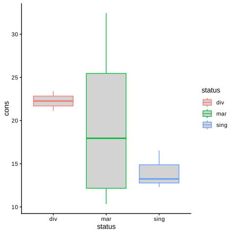
Figure 3.6: Box plot to check the equality of means
The conclusion will depend on whether the boxes are all overlapped or not. As we see, the div and sing boxes do not (with a significance level of 0.05), so we can conclude that the means are not equal. However, the mean of mar is significantly equal to both div and sing due to its large variability, which is an important issue, because the anova analysis requires the variances to be equal as an assumption.
Example 3.9 Let us generate the following data with only two variables, one continuous as a dependent variable, and the second one is of factor type as a regressor.
library(simglm)
set.seed(1133)
arguments <- list(
  formula = cons ~ 1 + status,
  fixed = list(status = list(
    var_type = 'factor', levels = c('sing', 'mar', 'div')
  )),
  error = list(variance = 4),
  sample_size = 30,
  reg_weights = c(2, 2.5, 0.7)
)

dat <- simulate_fixed(data = NULL, arguments) %>%
  simulate_error(arguments) %>%
  generate_response(arguments)

# keep only the the dependent variable and the dummy variables

dat <- dat[,c("cons", "status")]
head(dat)| cons | status |
|---|---|
| 3.3537307 | div |
| 4.8247590 | sing |
| 1.0313386 | sing |
| 7.1554922 | sing |
| 2.5342504 | sing |
| 0.1814665 | sing |
We can go ahead and fit the model.
| term | estimate | std.error | statistic | p.value |
|---|---|---|---|---|
| (Intercept) | 1.6755620 | 0.6622482 | 2.5301118 | 0.0175442 |
| statusmar | 2.8128160 | 0.9576093 | 2.9373315 | 0.0066960 |
| statusdiv | 0.7570396 | 1.0910598 | 0.6938571 | 0.4936988 |
As we see only one level is significant, statusmar. But as whole, we can say that the categorical variable status is significant.
The best approach to analyze this type of variables is by using the anova analysis. R provides an easy way to do this through the function aov.
| term | df | sumsq | meansq | statistic | p.value |
|---|---|---|---|---|---|
| status | 2 | 47.2645 | 23.632251 | 4.490372 | 0.0207235 |
| Residuals | 27 | 142.0975 | 5.262872 | NA | NA |
If we use the significance level of 0.05, we should reject the null hypothesis that the means are all equal, and hence the categorical variable has a significant effect.
This analysis assumes that the variances are equal. Let us thus compute those variances.
[out]     sing      mar      div
[out] 5.714665 3.821520 6.836839
The following test (among others) test this assumption5.
[out]
[out]   Bartlett test of homogeneity of variances
[out]
[out] data:  dat$cons by dat$status
[out] Bartlett's K-squared = 0.68771, df = 2, p-value = 0.709
With that p-value 0.709, we should not reject the null hypothesis that says the variances are equal, which justifies the use of the ANOVA results.
- We can obtain the ANOVA table by using the function
summary.aovwith the original model mod_dat as an argumentsummary.aov(mod_dat).
The function used to fit models with categorical variables is the same used for continuous ones, but we should first copy the data into python
import statsmodels.formula.api as smf

mod_py = smf.ols('cons~status', data=dat_py).fit()
result_py = mod_py.summary2().tables[1]
result_py| Coef. | Std.Err. | t | P>|t| | [0.025 ] | ||
|---|---|---|---|---|---|---|
| Intercept | 1.7326016 | 0.8670864 | 1.9981879 | 0.0558598 | -0.0465128 | 3.511716 |
| status[T.mar] | 2.7557764 | 1.1091807 | 2.4845153 | 0.0194687 | 0.4799256 | 5.031627 |
| status[T.sing] | 0.6429604 | 1.0910598 | 0.5892989 | 0.5605598 | -1.5957095 | 2.881630 |
And we retrieve the ANOVA table as follows:
import statsmodels.api as sm

# type=2 to get the result in a data frame
anova_py = sm.stats.anova_lm(mod_py, type=2)
anova_py| df | sum_sq | mean_sq | F | PR(>F) | |
|---|---|---|---|---|---|
| status | 2 | 40.29112 | 20.145561 | 3.827864 | 0.0343912 |
| Residual | 27 | 142.09755 | 5.262872 | NaN | NaN |
3.10.2 Regression with two categorical variables
For simplicity, we will include only two categorical variables, since the same analysis can be extended. Let us first include another categorical variable to the above data.
set.seed(1133)
arguments <- list(
  formula = cons ~ 1 + status+sex,
  fixed = list(status = list(var_type = 'factor', levels = c('sing', 'mar', 'div')), sex = list(var_type = 'factor', levels = c('female', 'male'))),
  error = list(variance = 4),
  sample_size = 30,
  reg_weights = c(2, 3.5, 2.5, 0.7)
)

dat_R <- simulate_fixed(data = NULL, arguments) %>%
  simulate_error(arguments) %>%
  generate_response(arguments)

# keep only the the dependent variable and the dummy variables
dat_R <- dat_R[,c("cons", "sex", "status")]
head(dat_R)| cons | sex | status |
|---|---|---|
| 5.012040 | female | div |
| 3.589554 | female | sing |
| 1.766998 | male | sing |
| 3.025467 | female | sing |
| 1.721436 | male | sing |
| 5.746511 | female | sing |
Before fitting the model, we should first visualize the distribution of the levels of each factor.
p1 <- ggplot(data = dat_R, aes(x = status, y = cons)) +
  geom_boxplot(fill = 'lightblue') +
  ggtitle('status') +
  theme_classic()

p2 <- ggplot(data = dat_R, aes(x = sex, y = cons)) +
  geom_boxplot(fill = 'yellow') +
  ggtitle('sex') +
  theme_classic()

# use patchwork package to concatenate the plots
p1 + p2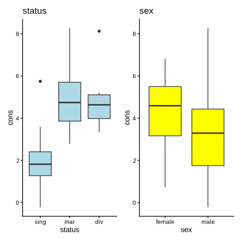
From the first plot, since the boxes do not overlap, we expect the factor status to be significant. Whereas the sex factor boxes overlap, indicating its non-significance in explaining the dependent variable cons.
Besides the separate effect of each factor, there exists another one that comes from the interaction between these factors. It can be visualized as follows:
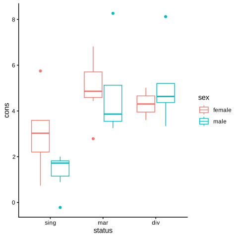
The first two boxes show that there is no significant difference between the divorced males and divorced females. The same conclusion applies to the second two boxes for married persons. However, the third two boxes show a slight separation between single males and single females. Since so, we cannot decide about interaction effect, and hence further statistic analysis is needed.
Let us verify this conclusion by fitting the model with the function lm.
| term | estimate | std.error | statistic | p.value |
|---|---|---|---|---|
| (Intercept) | 3.06 | 0.69 | 4.43 | 0.00 |
| sexmale | -1.71 | 0.90 | -1.89 | 0.07 |
| statusmar | 1.95 | 0.90 | 2.16 | 0.04 |
| statusdiv | 1.24 | 1.29 | 0.96 | 0.34 |
| sexmale:statusmar | 1.51 | 1.32 | 1.14 | 0.26 |
| sexmale:statusdiv | 2.54 | 1.58 | 1.61 | 0.12 |
If we have two factors, the first one with \(n\) levels and the second one with \(m\) levels, then the total number of dummies that we should create is \(n+m+(n\times m)\), where \((n\times m)\) for the interaction. But, as discussed in the previous subsection, we should remove some dummies to ensure the invertibility of the design matrix \(X\). In our case, for instance, The female and div levels are taken into account by the intercept, such that it remains male (from sex), mar and sing(from status), male-mar and male-sing (from interaction). To understand how the estimates computed, see the following formulation:
For females:
\[\begin{equation*} \widehat {cons}=\begin{cases} \overset{\Large\textit{ divorced female}}{\widehat\alpha_0+\widehat\alpha_1 \overbrace{mal}^{=0}+\widehat\beta_1 \overbrace{mar}^{=0}+\widehat\beta_2 \overbrace{sing}^{=0}+\widehat\gamma_1 \overbrace{malmar}^{=0}+\widehat\gamma_2 \overbrace{malsing}^{=0}=\widehat\alpha_0}\\ \overset{\Large\textit{married female}}{\widehat\alpha_0+\widehat\alpha_1 \overbrace{mal}^{=0}+\widehat\beta_1 \overbrace{mar}^{=1}+\widehat\beta_2 \overbrace{sing}^{=0}+\widehat\gamma_1 \overbrace{malmar}^{=0}+\widehat\gamma_2 \overbrace{malsing}^{=0}=\widehat\alpha_0+\widehat\beta_1}\\ \overset{\Large\textit{single female}}{\widehat\alpha_0+\widehat\alpha_1 \overbrace{mal}^{=0}+\widehat\beta_1 \overbrace{mar}^{=0}+\widehat\beta_2 \overbrace{sing}^{=1}+\widehat\gamma_1 \overbrace{malmar}^{=0}+\widehat\gamma_2 \overbrace{malsing}^{=0}=\widehat\alpha_0+\widehat\beta_2} \end{cases} \end{equation*}\]
- \(\widehat\alpha_0\): divorced female average.
- \(\widehat\beta_1\): married female average - divorced female average.
- \(\widehat\beta_2\): single female average - divorced female average.
For males:
\[\begin{equation*} \widehat {cons}=\begin{cases} \overset{\Large\textit{divorced male}}{\widehat\alpha_0+\widehat\alpha_1 \overbrace{mal}^{=1}+\widehat\beta_1 \overbrace{mar}^{=0}+\widehat\beta_2 \overbrace{sing}^{=0}+\widehat\gamma_1 \overbrace{malmar}^{=0}+\widehat\gamma_2 \overbrace{malsing}^{=0}=\widehat\alpha_0+\widehat\alpha_1}\\ \overset{\Large\textit{married male}}{\widehat\alpha_0+\widehat\alpha_1 \overbrace{mal}^{=1}+\widehat\beta_1 \overbrace{mar}^{=1}+\widehat\beta_2 \overbrace{sing}^{=0}+\widehat\gamma_1 \overbrace{malmar}^{=1}+\widehat\gamma_2 \overbrace{malsing}^{=0}=\widehat\alpha_0+\widehat\alpha_1+\widehat\beta_1+\widehat\gamma_1}\\ \overset{\Large\textit{single male}}{\widehat\alpha_0+\widehat\alpha_1 \overbrace{mal}^{=1}+\widehat\beta_1 \overbrace{mar}^{=0}+\widehat\beta_2 \overbrace{sing}^{=1}+\widehat\gamma_1 \overbrace{malmar}^{=0}+\widehat\gamma_2 \overbrace{malsing}^{=1}=\widehat\alpha_0+\widehat\alpha_1+\widehat\beta_2+\widehat\gamma_2} \end{cases} \end{equation*}\]
- \(\widehat\alpha_0+\widehat\alpha_1\): divorced male average.
- \(\widehat\beta_1+\widehat\gamma_1\): married male average - divorced male average.
- \(\widehat\beta_2+\widehat\gamma_2\): single male average - divorced male average.
Now let us verify these coefficients by comparing those averages from the data.
# compute the means
FFF <- tapply(dat_R$cons, list(dat_R$sex, dat_R$status), mean)

# convert the result into a long format
FFF <- as.data.frame.table(FFF)

# tidy the table
FFF$terms <- with(FFF, paste(Var1, Var2, sep = '-'))
FFF <- FFF[,c("terms", "Freq")]
names(FFF)[2]="means"
FFF| terms | means | |
|---|---|---|
| 1 | female-sing | 3.06 |
| 2 | male-sing | 1.35 |
| 3 | female-mar | 5.01 |
| 5 | female-div | 4.31 |
| 4 | male-mar | 4.81 |
| 6 | male-div | 5.13 |
DDD <- tidy(mod_R_2fac)
DDD <- DDD[,c("term", "estimate")]
# concatenate the two tables
GGG <- tibble(FFF, DDD)

# reorder the columns
GGG <- GGG[, c("terms", "term", "estimate", "means")]
GGG| terms | term | estimate | means |
|---|---|---|---|
| female-sing | (Intercept) | 3.06 | 3.06 |
| male-sing | sexmale | -1.71 | 1.35 |
| female-mar | statusmar | 1.95 | 5.01 |
| female-div | statusdiv | 1.24 | 4.31 |
| male-mar | sexmale:statusmar | 1.51 | 4.81 |
| male-div | sexmale:statusdiv | 2.54 | 5.13 |
Using that table, we can figure out how the coefficients have been computed:
- \(\widehat\alpha_0=\) divorced female average = \(1.81\).
- \(\widehat\beta_1=\) married female average - divorced female average=\(5.01-1.81=3.2\).
- \(\widehat\beta_2=\) single female average - divorced female average=\(5.56-1.81=3.75\).
- \(\widehat\alpha_1=\) divorced male average \(-\widehat\alpha_0=2.63-1.81=0.82\).
- \(\widehat\gamma_1=\) (married male average - divorced male average) \(-\widehat\beta_1=(4.81-2.63)-3.2=-1.02\).
- \(\widehat\gamma_2=\) (single male average - divorced male average) \(-\widehat\beta_2=(3.85-2.63)-3.75=-2.53\).
That said, let us now check the significance of those factors and their interaction. By using the lm function, we get:
| term | estimate | std.error | statistic | p.value |
|---|---|---|---|---|
| (Intercept) | 3.06 | 0.69 | 4.43 | 0.00 |
| sexmale | -1.71 | 0.90 | -1.89 | 0.07 |
| statusmar | 1.95 | 0.90 | 2.16 | 0.04 |
| statusdiv | 1.24 | 1.29 | 0.96 | 0.34 |
| sexmale:statusmar | 1.51 | 1.32 | 1.14 | 0.26 |
| sexmale:statusdiv | 2.54 | 1.58 | 1.61 | 0.12 |
Using the level of 0.05, the interaction effect is not significant since the Intercept (p-value=0.11), the sexmale:statusmar (p-value=0.53), and the sexmale:statussing (p-value=0.12) are all not significant. The factor sex is also non-significant because, in addition to the non-significance intercept, the sexmale level (p-value=0.53) is not significant. However, the only significant regressor is the factor status.
When, however, we use the ANOVA table the interpretation is straightforward as follows.
| term | df | sumsq | meansq | statistic | p.value |
|---|---|---|---|---|---|
| sex | 1 | 4.96 | 4.96 | 2.08 | 0.16 |
| status | 2 | 56.56 | 28.28 | 11.86 | 0.00 |
| sex:status | 2 | 6.91 | 3.46 | 1.45 | 0.25 |
| Residuals | 24 | 57.21 | 2.38 | NA | NA |
As we can see, by looking at the p.value, we can conclude that the only significant effect comes from the categorical variable status without any interaction with the variable sex.
To correct our model, we should remove the non-significant term from the model one by one, but should start first with the interaction term then check again until we left out with only significant ones.
| term | estimate | std.error | statistic | p.value |
|---|---|---|---|---|
| (Intercept) | 2.43 | 0.57 | 4.24 | 0.00 |
| sexmale | -0.63 | 0.60 | -1.05 | 0.31 |
| statusmar | 2.74 | 0.67 | 4.09 | 0.00 |
| statusdiv | 2.92 | 0.75 | 3.88 | 0.00 |
Even though the sexmale term is non-significant, we cannot remove the sex variable since the intercept is significant so that we we do not know, from this output, if that significance comes from status or sex or from both. That is why whe need the ANOVA table to clear up this confusion.
| term | df | sumsq | meansq | statistic | p.value |
|---|---|---|---|---|---|
| sex | 1 | 4.96 | 4.96 | 2.01 | 0.17 |
| status | 2 | 56.56 | 28.28 | 11.47 | 0.00 |
| Residuals | 26 | 64.13 | 2.47 | NA | NA |
It is clear now that the variable sex is also non-significant and should be removed.
In python, after retrieving the data from R, we can visualize the box plots using seaborn package.
copy the data into python.
import matplotlib.pyplot as plt
import seaborn as sns

# create placeholder for the plots
fig = plt.figure(figsize=(15,15))
g = plt.GridSpec(2,2, wspace=0.4, hspace=0.4)
ax1 = fig.add_subplot(g[0,0])
ax2 = fig.add_subplot(g[0,1])
ax3 = fig.add_subplot(g[1,0:])

# boxplot for status
sns.boxplot(x='status', y= 'cons', data=data_py, ax=ax1)

# boxplot fro sex
sns.boxplot(x='sex', y= 'cons', data=data_py, ax=ax2)

# interaction
sns.boxplot(x='status', y= 'cons', hue='sex', data=data_py, ax=ax3)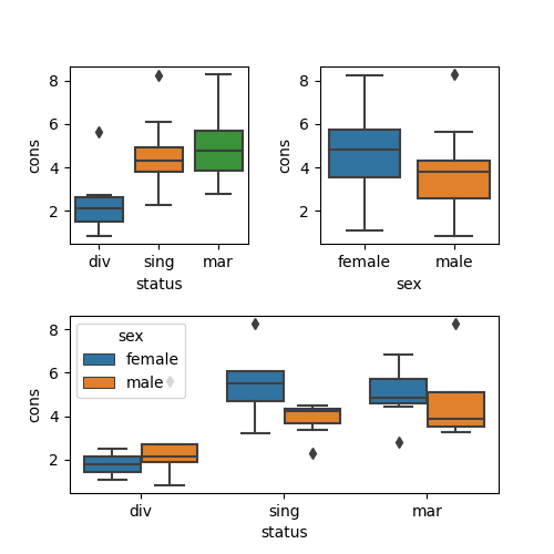
The following code fragment is for the estimation.
mod_py_2factor = smf.ols('cons~sex*status', data=data_py).fit()
result2_py= mod_py_2factor.summary2().tables[1]
result2_py| Coef. | Std.Err. | t | P>|t| | [0.025 ] | ||
|---|---|---|---|---|---|---|
| Intercept | 1.81 | 1.09 | 1.65 | 0.11 | -0.45 | 4.06 |
| sex[T.male] | 0.83 | 1.29 | 0.64 | 0.53 | -1.84 | 3.49 |
| status[T.mar] | 3.20 | 1.24 | 2.59 | 0.02 | 0.65 | 5.76 |
| status[T.sing] | 3.76 | 1.29 | 2.91 | 0.01 | 1.09 | 6.42 |
| sex[T.male]:status[T.mar] | -1.03 | 1.61 | -0.64 | 0.53 | -4.36 | 2.31 |
| sex[T.male]:status[T.sing] | -2.54 | 1.58 | -1.61 | 0.12 | -5.79 | 0.72 |
And the ANOVA table can be retrieved by the following:
| df | sum_sq | mean_sq | F | PR(>F) | |
|---|---|---|---|---|---|
| sex | 1 | 8.05 | 8.05 | 3.38 | 0.08 |
| status | 2 | 24.97 | 12.48 | 5.24 | 0.01 |
| sex:status | 2 | 6.91 | 3.46 | 1.45 | 0.25 |
| Residual | 24 | 57.21 | 2.38 | NaN | NaN |
3.10.3 Regression with mix of categorical and continuous variables
This analysis called ANCOVA in the econometric jargon. We will use again the above example with the variable income added as continuous independent variable.
set.seed(1133)
arguments <- list(
  formula = cons ~ 1 + income * sex,
  fixed = list(
    income = list(
      var_type = 'continuous',
      mean = 150,
      sd = 5
    ),
    sex = list(var_type = 'factor', levels = c('female', 'male'))
  ),
  error = list(variance = 4),
  sample_size = 30,
  reg_weights = c(8, 0.65,-0.7, 0.4)
)

dat2_R <- simulate_fixed(data = NULL, arguments) %>%
  simulate_error(arguments) %>%
  generate_response(arguments)

# keep only the the dependent variable and the dummy variables
dat2_R <- dat2_R[,c("cons",  "income", "sex")]
head(dat2_R)| cons | income | sex |
|---|---|---|
| 108.5085 | 156.617 | female |
| 108.2729 | 155.336 | female |
| 162.1956 | 147.515 | male |
| 157.9419 | 146.278 | male |
| 104.2982 | 150.930 | female |
| 169.2698 | 155.270 | male |
Now let us figure out how these coefficient have been computed.
| (Intercept) | income | sexmale | income:sexmale |
|---|---|---|---|
| 1 | 156.617 | 0 | 0.000 |
| 1 | 155.336 | 0 | 0.000 |
| 1 | 147.515 | 1 | 147.515 |
| 1 | 146.278 | 1 | 146.278 |
| 1 | 150.930 | 0 | 0.000 |
| 1 | 155.270 | 1 | 155.270 |
The model creates three regressors from the two original ones. While we know how is sexmale generated from the earlier discussion, we do not yet know for the third variable income:sexmale. It turns out that income:sexmale gives two slopes, each for each level of the factor sex. The following formula should clear up what is going on.
\[\begin{equation*} \widehat {cons}=\begin{cases} \overset{\Large\textit{Regression equation for females}}{\widehat\alpha_0+\widehat\alpha_1 inc+\widehat\beta \overbrace{mal}^{=0}+\widehat\gamma \overbrace{incmale}^{=0}=\widehat\alpha_0+\widehat\alpha_1 inc}\\ \overset{\Large\textit{Regression equation for males}}{\widehat\alpha_0+\widehat\alpha_1 inc+\widehat\beta \overbrace{mal}^{=1}+\widehat\gamma \overbrace{incmale}^{=inc}=(\widehat\alpha_0+\widehat\beta)+(\widehat\alpha_1+\widehat\gamma) inc}\\ \end{cases} \end{equation*}\]
Now the interpretation is straightforward. The model gives two fitted lines, one for each factor level, and their relationship determines the significance of the different terms. That yields six possible situations where the two trivial ones are (assuming that all the remaining coefficients are significant):
- \(\widehat\beta\approx0\) and \(\widehat\gamma\approx0\): The variable sex does not affect at all the response variable.
- \(\widehat\alpha_1\approx0\) and \(\widehat\gamma\approx0\): The variable income has no effect on the response variable.
All the other situations englobe the significance of each level and the interaction term. For instance, if only \(\widehat\gamma\approx0\), we do not have the interaction term between the two regressors. In other words, the effect of income on the response is the same whether the associated individual is male or female.
| term | estimate | std.error | statistic | p.value |
|---|---|---|---|---|
| (Intercept) | -10.446 | 15.027 | -0.695 | 0.493 |
| income | 0.769 | 0.098 | 7.833 | 0.000 |
| sexmale | 11.279 | 19.281 | 0.585 | 0.564 |
| income:sexmale | 0.321 | 0.127 | 2.525 | 0.018 |
Since \(\widehat\alpha_0\) and \(\widehat\beta\) are non-significant, we have two lines without intercept but with different slopes, the slope for females is \(\widehat\alpha_1=0.769\), whereas for males is \(\widehat\alpha_1+\widehat\gamma=0.769+0.321=1.09\).
The above table displays the effect size of each term. If we want to check only the significance of the regressors included in the model, we should use the function aov to display the ANCOVA table that shows the significance of each variable with their interaction as well.
| term | df | sumsq | meansq | statistic | p.value |
|---|---|---|---|---|---|
| income | 1 | 305.960 | 305.960 | 83.989 | 0.000 |
| sex | 1 | 24607.138 | 24607.138 | 6754.870 | 0.000 |
| income:sex | 1 | 23.226 | 23.226 | 6.376 | 0.018 |
| Residuals | 26 | 94.715 | 3.643 | NA | NA |
Now it is clear that the two variables with their interaction are significant. Lastly, we can visualize these two fitted lines as follows:
ggplot(dat2_R, aes(x=income, y=cons, color=sex))+
  geom_point()+
  geom_smooth(method='lm', se=FALSE)+
  ylab('consumption')+
  xlab('income')+
theme_classic() 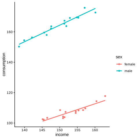
First, we have to send a copy of the data to Python workspace.
Then we can fit the model.
import statsmodels.formula.api as smf

# fit the model
mod_py_ancova= smf.ols('cons~inc*sex', data=dat2_py).fit()
mod_result =mod_py_ancova.summary2().tables[1]
mod_result| Coef. | Std.Err. | t | P>|t| | [0.025 ] | ||
|---|---|---|---|---|---|---|
| Intercept | -10.446 | 15.027 | -0.695 | 0.493 | -41.334 | 20.443 |
| sex[T.male] | 11.279 | 19.281 | 0.585 | 0.564 | -28.352 | 50.911 |
| inc | 0.769 | 0.098 | 7.833 | 0.000 | 0.567 | 0.971 |
| inc:sex[T.male] | 0.321 | 0.127 | 2.525 | 0.018 | 0.060 | 0.582 |
Then, we can retrieve the ANCOVA table with the following script.
| df | sum_sq | mean_sq | F | PR(>F) | |
|---|---|---|---|---|---|
| sex | 1 | 24048.60 | 24048.60 | 6601.55 | 0.00 |
| inc | 1 | 864.50 | 864.50 | 237.31 | 0.00 |
| inc:sex | 1 | 23.23 | 23.23 | 6.38 | 0.02 |
| Residual | 26 | 94.71 | 3.64 | NaN | NaN |
we will discuss the heteroskedasticity assumption in later chapters↩︎