7.2 Stationarity
A stochastic process is stationary if the joint distribution of \(\{X_{t-1+h},...,X_{t-n+h}\}\) is identical to the join distribution of \(\{X_{t-1},...,X_{t-n}\}\). That is:
\[\begin{equation} F\Big(X_{t-1+h},...,X_{t-n+h}\Big)=F\Big(X_{t-1},...,X_{t-n}\Big) \end{equation}\]
If all the moments of a stationary process are independent of time, then this process is called strongly stationary. However, if some higher-order moments are not independent of time, then we are talking about weak stationary process. In most economic studies, we need only a weakly stationary process of order two. That is, we need only the independence of the mean and the covariance. White noise is a basic example of a weak stationary process.
\[\begin{align} &E(X_t)=\mu \\ &Var(X_t)=E\big[(X_t-\mu)(X_t-\mu)^t\big]=\sigma^2 \\ &cov(X_t-X_{t-k})=E\big[(X_t-\mu)(X_{t-k}-\mu)^t\big]=\gamma_k \end{align}\]
In other words, we say that our time series is stationary if this time series does not have any trend or seasonality or any other component that has some fixed pattern over time.
We have two types of non stationary time series
TS (Trend stationary):
We encounter this type when the time series has a deterministic component (trend) so that its mean is dependent of time. Formally, it can be written:
\[\begin{align} &X_t=f_t+\varepsilon_t \\ &E(X_t)=E(f_t)+\overbrace{E(\varepsilon_t)}^{=0}=\mu_t \end{align}\]
Where \(f_t\) is a function (linear or non linear) of time, and \(\varepsilon_t\) is a white noise.
This type of process can be transformed into a stationary time series by subtracting the original time series \(X_t\) from the fitted time series \(\hat X_t\). For instance, if \(f_t=\beta_O+\beta_1 t\), then \(Z_t=X_t-\hat\beta_0-\hat\beta_1t\) will be stationary process because:
\[\begin{align} E\Big[X_t-\hat\beta_0-\hat\beta_1t\Big]&=E\Big[\beta_0+\beta_1t+\varepsilon_t-\hat\beta_0-\hat\beta_1t\Big] \\ &=\overbrace{E(\beta_0-\hat\beta_0)}^{=0}+\overbrace{E(\beta_1-\hat\beta_1)}^{=0}t+\overbrace{E(\varepsilon_t)}^{=0} \\ &=0 \end{align}\]
DS (Differency stationary):
The random walk discussed earlier ((7.7)) is non stationary of type DS (first difference). By taking the difference between the current value and the lagged value, the resulted process will be stationary.
\[\begin{equation} X_t-X_{t-1}=\varepsilon_t \end{equation}\]
7.2.1 Unit root
Let us go back to the first order auto-regressive process and write it without any constant:
\[\begin{equation} y_t=\phi y_{t-1}+\varepsilon_t \tag{7.27} \end{equation}\]
We have seen that this process is stationary as long as \(\lvert\phi\rvert<1\), because in that case the variance converges towards \(\frac{\sigma^2}{1-\phi^2}\). The borderline case \(\phi=1\) deserves a particular attention, since it turns the process into the random walk of equation (7.7). Using the lag operator, the process is written \((1-\phi D)y_t=\varepsilon_t\), and its characteristic equation \(1-\phi D=0\) admits the root \(D=\frac{1}{\phi}\). When \(\phi=1\) this root is equal to one, it lies on the unit circle instead of outside it, and this is the reason why we say that the process has a unit root.
The consequence of a unit root is that a shock never dies out. Writing the random walk recursively gives \(y_t=y_0+\sum_{i=1}^{t}\varepsilon_i\), so that the variance \(Var(y_t)=t\sigma^2\) grows without bound with time, and the series has no mean to which it can return. Regressing two independent series of this kind on each other produces the well known problem of spurious regression, where the \(R^2\) and the Student statistics suggest a strong relation that does not exist.
It is tempting to test \(\phi=1\) with the usual Student statistic of the OLS estimator. Unfortunately, under the null hypothesis of a unit root the series is not stationary, the classical asymptotic results no longer hold, and this statistic does not follow a Student distribution. Dickey and Fuller have derived the correct distribution, and all the tests presented in this section rely on it, or on some refinement of it.
To illustrate them, we simulate two series with the same length: a random walk, which has a unit root by construction, and a stationary \(AR(1)\) with \(\phi=0.5\).
In R:
set.seed(123)

# a random walk: phi = 1
rw_ts <- ts(cumsum(rnorm(300)))

# a stationary AR(1): phi = 0.5
ar_ts <- ts(arima.sim(model = list(ar = 0.5), n = 300))

# plot both series
par(mfrow = c(1, 2))
plot(rw_ts, main = "Random walk", ylab = "")
plot(ar_ts, main = "Stationary AR(1)", ylab = "")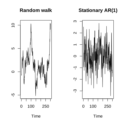
Figure 7.12: a random walk and a stationary AR(1)
The difference is visible to the naked eye. The random walk wanders away without ever coming back, while the \(AR(1)\) keeps crossing its own mean. The tests that follow put a formal decision behind this visual impression.
7.2.1.1 Dickey-Fuller test
The trick of Dickey and Fuller is to subtract \(y_{t-1}\) from both sides of equation (7.27):
\[\begin{align} y_t-y_{t-1}&=\phi y_{t-1}-y_{t-1}+\varepsilon_t \\ \vartriangle y_t&=(\phi-1)y_{t-1}+\varepsilon_t \\ \vartriangle y_t&=\delta y_{t-1}+\varepsilon_t \tag{7.28} \end{align}\]
Testing \(\phi=1\) becomes then equivalent to testing \(\delta=0\), and the hypotheses of the test are:
\[\begin{align} &H_0: \delta=0 \quad \text{the series has a unit root (non stationary)} \\ &H_1: \delta<0 \quad \text{the series is stationary} \end{align}\]
The test is one sided, because a value \(\phi>1\) would give an explosive process that we rule out from the start. Since the statistic does not follow a Student distribution, it is compared to the critical values tabulated by Dickey and Fuller, which are more negative than the usual ones.
Three specifications are used in practice, and the choice between them is not innocent. Adding a term that does not belong to the data generating process costs power, while omitting one that does belong biases the test towards the non rejection of the unit root:
without constant and without trend: \(\vartriangle y_t=\delta y_{t-1}+\varepsilon_t\)
with a constant: \(\vartriangle y_t=\alpha+\delta y_{t-1}+\varepsilon_t\)
with a constant and a trend: \(\vartriangle y_t=\alpha+\beta t+\delta y_{t-1}+\varepsilon_t\)
The R package urca gives access to the three specifications through the argument type, and prints the statistic together with the critical values.
In R:
library(urca)

# Dickey-Fuller test (lags = 0) with a constant, on the random walk
df_rw <- ur.df(rw_ts, type = "drift", lags = 0)
summary(df_rw)
#>
#> ###############################################
#> # Augmented Dickey-Fuller Test Unit Root Test #
#> ###############################################
#>
#> Test regression drift
#>
#>
#> Call:
#> lm(formula = z.diff ~ z.lag.1 + 1)
#>
#> Residuals:
#> Min 1Q Median 3Q Max
#> -2.21024 -0.65060 -0.04459 0.56844 2.98635
#>
#> Coefficients:
#> Estimate Std. Error t value Pr(>|t|)
#> (Intercept) 0.09999 0.06189 1.616 0.1072
#> z.lag.1 -0.04253 0.01972 -2.156 0.0319 *
#> ---
#> Signif. codes: 0 '***' 0.001 '**' 0.01 '*' 0.05 '.' 0.1 ' ' 1
#>
#> Residual standard error: 0.941 on 297 degrees of freedom
#> Multiple R-squared: 0.01541, Adjusted R-squared: 0.0121
#> F-statistic: 4.65 on 1 and 297 DF, p-value: 0.03186
#>
#>
#> Value of test-statistic is: -2.1564 2.549
#>
#> Critical values for test statistics:
#> 1pct 5pct 10pct
#> tau2 -3.44 -2.87 -2.57
#> phi1 6.47 4.61 3.79The statistic of interest is the first one, tau2. Its value is far above (less negative than) the critical value at the 5% level, so we cannot reject the null hypothesis: the random walk does have a unit root, which is what we built it for. Let us now apply the same test to the stationary series.
# the same test on the stationary AR(1)
df_ar <- ur.df(ar_ts, type = "drift", lags = 0)
summary(df_ar)
#>
#> ###############################################
#> # Augmented Dickey-Fuller Test Unit Root Test #
#> ###############################################
#>
#> Test regression drift
#>
#>
#> Call:
#> lm(formula = z.diff ~ z.lag.1 + 1)
#>
#> Residuals:
#> Min 1Q Median 3Q Max
#> -2.93901 -0.58256 -0.00769 0.64378 2.45679
#>
#> Coefficients:
#> Estimate Std. Error t value Pr(>|t|)
#> (Intercept) 0.004255 0.056310 0.076 0.94
#> z.lag.1 -0.602209 0.052855 -11.394 <2e-16 ***
#> ---
#> Signif. codes: 0 '***' 0.001 '**' 0.01 '*' 0.05 '.' 0.1 ' ' 1
#>
#> Residual standard error: 0.9733 on 297 degrees of freedom
#> Multiple R-squared: 0.3041, Adjusted R-squared: 0.3018
#> F-statistic: 129.8 on 1 and 297 DF, p-value: < 2.2e-16
#>
#>
#> Value of test-statistic is: -11.3936 64.9352
#>
#> Critical values for test statistics:
#> 1pct 5pct 10pct
#> tau2 -3.44 -2.87 -2.57
#> phi1 6.47 4.61 3.79This time the statistic is clearly below the critical value, and the null hypothesis of a unit root is rejected. The test recognizes the stationary series.
7.2.1.2 Augmented Dickey-Fuller test
The Dickey-Fuller test assumes that the errors of equation (7.28) are a white noise. This assumption is rarely satisfied with real data, where the series usually carries a richer dynamic than a simple \(AR(1)\). If the residuals remain autocorrelated, the statistic is biased and the conclusion cannot be trusted.
The solution proposed by Dickey and Fuller themselves is to augment the regression with the lagged differences of the series, so that they absorb the remaining dynamic and leave a white noise behind:
\[\begin{equation} \vartriangle y_t=\alpha+\beta t+\delta y_{t-1}+\sum_{i=1}^{p}\gamma_i \vartriangle y_{t-i}+\varepsilon_t \tag{7.29} \end{equation}\]
The hypotheses are unchanged, and so are the critical values. The only new question is the number of lags \(p\). Choosing it too small leaves autocorrelation in the residuals, and choosing it too large wastes observations. In practice we select it with an information criterion such as the \(AIC\) or the \(BIC\), which is what the argument selectlags does.
In R:
# the number of lags is chosen by the AIC
adf_rw <- ur.df(rw_ts, type = "drift", selectlags = "AIC")
adf_ar <- ur.df(ar_ts, type = "drift", selectlags = "AIC")

# we collect only the statistics and the critical values
adf_out <- data.frame(
  series    = c("random walk", "stationary AR(1)"),
  statistic = c(adf_rw@teststat[1], adf_ar@teststat[1]),
  crit_5pct = c(adf_rw@cval[1, "5pct"], adf_ar@cval[1, "5pct"])
)
adf_out$decision <- ifelse(adf_out$statistic < adf_out$crit_5pct,
                           "reject H0 : stationary",
"do not reject H0 : unit root")| series | statistic | crit_5pct | decision |
|---|---|---|---|
| random walk | -2.107 | -2.87 | do not reject H0 : unit root |
| stationary AR(1) | -9.647 | -2.87 | reject H0 : stationary |
The conclusion is the same as before, but it is now robust to a possible autocorrelation of the errors.
In Python:
We move the two series to python, and we use the function adfuller of the statsmodels package. It returns the statistic, the p-value, the number of lags retained, the number of observations used and a dictionary of critical values.
import pandas as pd
from statsmodels.tsa.stattools import adfuller

def adf_row(name, x):
    stat, pval, lags, nobs, crit, _ = adfuller(x, regression="c", autolag="AIC")
    return {"series": name, "statistic": round(stat, 3), "p_value": round(pval, 4),
            "lags": lags, "crit_5pct": round(crit["5%"], 3)}

adf_py = pd.DataFrame([adf_row("random walk", rw_py),
adf_row("stationary AR(1)", ar_py)])| series | statistic | p_value | lags | crit_5pct |
|---|---|---|---|---|
| random walk | -2.156 | 0.2225 | 0 | -2.871 |
| stationary AR(1) | -11.394 | 0.0000 | 0 | -2.871 |
The p-value makes the reading immediate: it is large for the random walk, so the unit root is not rejected, and it is very small for the \(AR(1)\), so it is rejected.
7.2.1.3 Philip Perron test
Phillips and Perron reach the same objective as the augmented test, but by a different road. Instead of adding lagged differences to the regression, they keep the simple specification of equation (7.28) and correct the statistic afterwards, in a non parametric way, for the autocorrelation and the possible heteroskedasticity of the errors. The correction uses a long run variance estimated with a Newey-West type window:
\[\begin{equation} \sigma_{lr}^2=\gamma_0+2\sum_{j=1}^{l}\Big(1-\frac{j}{l+1}\Big)\gamma_j \tag{7.30} \end{equation}\]
where \(\gamma_j\) is the autocovariance of the residuals at the lag \(j\) and \(l\) is the truncation lag. The hypotheses and the critical values remain those of Dickey and Fuller. The advantage of this test is that it does not require us to choose a number of lags for the regression itself, and it behaves well when the errors are heteroskedastic. Its drawback is a poor behaviour when the series contains a strong negative moving average component.
In R:
library(tseries)

pp_rw <- pp.test(rw_ts)
pp_ar <- pp.test(ar_ts)

pp_out <- data.frame(
  series    = c("random walk", "stationary AR(1)"),
  statistic = c(pp_rw$statistic, pp_ar$statistic),
  p_value   = c(pp_rw$p.value, pp_ar$p.value)
)| series | statistic | p_value |
|---|---|---|
| random walk | -11.1946 | 0.4827 |
| stationary AR(1) | -179.3897 | 0.0100 |
In Python:
The statsmodels package does not provide this test, so we use the arch package, which gathers the whole family of unit root tests in the module arch.unitroot.
from arch.unitroot import PhillipsPerron

pp_py = pd.DataFrame([
    {"series": "random walk",
     "statistic": round(PhillipsPerron(rw_py).stat, 3),
     "p_value": round(PhillipsPerron(rw_py).pvalue, 4)},
    {"series": "stationary AR(1)",
     "statistic": round(PhillipsPerron(ar_py).stat, 3),
     "p_value": round(PhillipsPerron(ar_py).pvalue, 4)}
])| series | statistic | p_value |
|---|---|---|
| random walk | -2.288 | 0.1757 |
| stationary AR(1) | -11.487 | 0.0000 |
7.2.1.4 Kpss test
The three previous tests share the same null hypothesis, the presence of a unit root. This is not a neutral choice. A statistical test never proves the null hypothesis, it only fails to reject it, and these tests are known to have a low power when \(\phi\) is close to one without being equal to it. Concluding “we did not reject the unit root” is therefore a much weaker statement than it looks.
Kwiatkowski, Phillips, Schmidt and Shin proposed a test that reverses the hypotheses. The series is decomposed into a deterministic trend, a random walk and a stationary error:
\[\begin{equation} y_t=\xi t+r_t+\varepsilon_t \quad \text{with} \quad r_t=r_{t-1}+u_t \tag{7.31} \end{equation}\]
The series is stationary if and only if the random walk component is in fact constant, that is if the variance of \(u_t\) is null. The hypotheses become:
\[\begin{align} &H_0: \sigma_u^2=0 \quad \text{the series is stationary} \\ &H_1: \sigma_u^2>0 \quad \text{the series has a unit root} \end{align}\]
Note that a large statistic now leads to the rejection of stationarity, which is the opposite of what we did with the previous tests. The usual practice is to apply the KPSS test together with the augmented Dickey-Fuller test and to read the two conclusions jointly:
ADF rejects and KPSS does not reject: the series is stationary.
ADF does not reject and KPSS rejects: the series has a unit root.
both reject, or neither rejects: the result is not conclusive, and the series probably needs a closer look.
In R:
kpss_rw <- kpss.test(rw_ts, null = "Level")
kpss_ar <- kpss.test(ar_ts, null = "Level")

kpss_out <- data.frame(
  series    = c("random walk", "stationary AR(1)"),
  statistic = c(kpss_rw$statistic, kpss_ar$statistic),
  p_value   = c(kpss_rw$p.value, kpss_ar$p.value)
)| series | statistic | p_value |
|---|---|---|
| random walk | 0.4856 | 0.0449 |
| stationary AR(1) | 0.1410 | 0.1000 |
The p-value of the random walk is small, so stationarity is rejected, while the one of the \(AR(1)\) is large, so stationarity is not rejected. Read together with the augmented Dickey-Fuller test, the two series fall exactly into the first two cases of the list above.
In Python:
from statsmodels.tsa.stattools import kpss

# the two languages do not choose the same number of lags by default, so we
# impose here the rule used by R, trunc(4*(n/100)^(1/4)), to make the two
# tables comparable.
def kpss_row(name, x):
    nlag = int(4 * (len(x) / 100) ** 0.25)
    stat, pval, lags, crit = kpss(x, regression="c", nlags=nlag)
    return {"series": name, "statistic": round(stat, 4),
            "p_value": round(pval, 4), "crit_5pct": crit["5%"]}

kpss_py = pd.DataFrame([kpss_row("random walk", rw_py),
kpss_row("stationary AR(1)", ar_py)])| series | statistic | p_value | crit_5pct |
|---|---|---|---|
| random walk | 0.4856 | 0.0449 | 0.463 |
| stationary AR(1) | 0.1410 | 0.1000 | 0.463 |
The number of lags used to estimate the long run variance has a real influence on the result. With too many lags the statistic is shrunk towards zero and the test loses the ability to detect the unit root, which is why the two languages must be given the same rule before their outputs can be compared.
The p-value returned by these functions is interpolated inside a table of critical values. When the statistic falls outside that table, the function returns the closest bound and warns that the true p-value is smaller, or greater, than the one printed. The warning is not an error, it only reminds us that the exact value is unknown.
7.2.2 Autocorrelation function ACF
The correlogram introduced earlier is not only a tool for identifying the order of a process, it is also the quickest way to recognize a non stationary series before running any test.
For a stationary process, we have shown that the autocorrelations decrease geometrically, \(\gamma_k=\phi^k\), and since \(\lvert\phi\rvert<1\) they vanish quickly. For a series with a unit root the picture is completely different. The correlation between \(y_t\) and \(y_{t-k}\) stays very close to one whatever the lag, and the correlogram decays in an almost linear way instead of dying out. This very slow decay is the visual signature of a unit root.
In R:
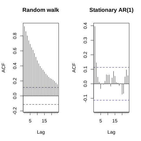
Figure 7.13: correlogram of a non stationary and a stationary series
The contrast is striking. The correlogram of the random walk stays outside the confidence band for a very long time, while the one of the \(AR(1)\) falls inside it after the second lag.
Once the series is differenced, the same correlogram should collapse immediately, which confirms that one difference was enough to remove the unit root.
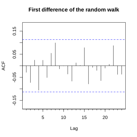
Figure 7.14: correlogram of the differenced random walk
There is no spike left outside the confidence band, so the differenced series behaves as a white noise, exactly as the theory predicts since \(\vartriangle y_t=\varepsilon_t\).
7.2.3 Partiall autocorrelation function PACF
The partial correlogram completes the diagnosis. For a series with a unit root it shows one very large spike at the first lag, close to one, and almost nothing afterwards, because the whole memory of the process passes through \(y_{t-1}\).
In R:
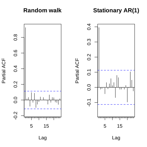
Figure 7.15: partial correlogram of a non stationary and a stationary series
Both series show a single spike, but the one of the random walk is much closer to one, which is the value of \(\phi\) that produces the unit root.
In practice the two correlograms are read together with the unit root tests, and they are used in this order: the plots suggest whether the series has to be differenced, the tests confirm it, and once the series is made stationary the same plots serve again to choose the orders \(p\) and \(q\) of the model, according to the mirror rule given in the previous section. This is exactly the identification step of the methodology that we develop in the next section.