8.4 Imputing missing values
Real data have holes. An indicator was not collected that year, a respondent skipped a question, a sensor failed for a week. Almost every algorithm of this chapter refuses a matrix containing missing values, so something must be done before modelling, and that something is not innocent.
The first question is why the value is missing, because the answer determines what is legitimate. Rubin’s classical distinction has three cases:
MCAR, missing completely at random: the probability of being missing does not depend on anything. Deleting the incomplete rows then loses precision but introduces no bias.
MAR, missing at random: the probability depends on the observed variables, for instance the income is missing more often for the young, but not on the missing value itself once age is known. Imputation using the other variables is valid here, and this is the case the usual methods assume.
MNAR, missing not at random: the probability depends on the unobserved value itself, for instance high incomes are hidden precisely because they are high. No method can repair this from the data alone, and a model of the missing mechanism is required.
The simplest remedies are also the worst. Deleting every incomplete row can destroy most of the sample when the holes are scattered, and it biases the results as soon as we leave the MCAR case. Replacing a hole by the mean of the column keeps the sample size but shrinks the variance and flattens the correlations, since every imputed point sits exactly at the centre.
The better approaches use the relations between variables. Imputation by a model predicts the missing variable from the others, for instance by a regression or by nearest neighbours. Multiple imputation goes one step further: it produces several complete data sets, each with a different draw of the missing values, analyses them separately and combines the results, so that the uncertainty due to the imputation is carried into the final standard errors instead of being ignored.
In R:
set.seed(123)
n <- 300
xi <- rnorm(n)
yi <- 1.5 * xi + rnorm(n, sd = .7)
full <- data.frame(x = xi, y = yi)

# a MAR mechanism: y disappears more often when x is large
miss <- runif(n) < plogis(1.6 * xi - 0.7)
obs <- full; obs$y[miss] <- NA
cat("share of missing values:", round(mean(miss), 3), "\n")
#> share of missing values: 0.36# three strategies
mean_imp <- obs; mean_imp$y[is.na(mean_imp$y)] <- mean(obs$y, na.rm = TRUE)
reg_fit <- lm(y ~ x, data = obs)
reg_imp <- obs; reg_imp$y[is.na(obs$y)] <- predict(reg_fit, newdata = obs[is.na(obs$y), ])
dd <- rbind(
data.frame(full, kind = "1. complete data (unknown)"),
data.frame(obs[!is.na(obs$y), ], kind = "2. listwise deletion"),
data.frame(mean_imp, kind = "3. mean imputation"),
data.frame(reg_imp, kind = "4. regression imputation"))
ggplot(dd, aes(x, y)) +
geom_point(alpha = .45, size = .9, colour = "grey30") +
geom_smooth(method = "lm", se = FALSE, colour = "firebrick", linewidth = .8) +
facet_wrap(~ kind, nrow = 1) +
labs(title = "the same data under four treatments of the holes") +
theme_minimal()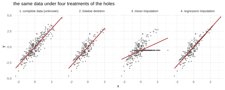
Figure 8.61: what each imputation does to the joint distribution
The four panels show what is at stake. The first is the truth, which we would never observe. The second keeps only the complete rows, and since the holes are concentrated on the right the cloud loses that region entirely. The third places every imputed point on a horizontal line at the mean, an artefact that is visible to the naked eye and that flattens the slope. The fourth puts them exactly on the regression line, which preserves the slope but suppresses the dispersion: the imputed points are too well behaved.
suppressPackageStartupMessages(library(mice))

# multiple imputation: 5 complete data sets, analysed and pooled
mi  <- mice(obs, m = 5, method = "pmm", printFlag = FALSE, seed = 1)
fit_mi <- with(mi, lm(y ~ x))
pooled <- summary(pool(fit_mi))

slope <- function(d) coef(lm(y ~ x, data = d))[2]
se_of <- function(d) summary(lm(y ~ x, data = d))$coefficients[2, 2]

comp_imp <- data.frame(
  method = c("complete data (unknown)", "listwise deletion", "mean imputation",
             "regression imputation", "multiple imputation"),
  slope = c(slope(full), slope(obs[!is.na(obs$y), ]), slope(mean_imp),
            slope(reg_imp), pooled$estimate[2]),
  std_error = c(se_of(full), se_of(obs[!is.na(obs$y), ]), se_of(mean_imp),
                se_of(reg_imp), pooled$std.error[2])
)| method | slope | std_error |
|---|---|---|
| complete data (unknown) | 1.4556 | 0.0423 |
| listwise deletion | 1.4733 | 0.0649 |
| mean imputation | 0.6089 | 0.0536 |
| regression imputation | 1.4733 | 0.0333 |
| multiple imputation | 1.4274 | 0.0501 |
The column of interest is the standard error as much as the slope. Regression imputation may land close to the true slope, but it reports a standard error that is too small, because it treats invented values as if they had been observed. Multiple imputation is built precisely to avoid that illusion: its standard error includes the variability between the imputed data sets, and is therefore the honest one.
Whatever the method, the imputation must be learned on the training set only and then applied to the test set. Computing a mean, or fitting an imputation model, on the whole data before splitting lets information from the test set leak into the training, and the measured performance becomes optimistic. The same rule applies to every transformation of the last section.