8.5 Models for outliers detection
An outlier is an observation that does not resemble the others. Behind that simple definition sit two very different situations, and confusing them is a frequent mistake.
Sometimes the outlier is an error: a decimal point misplaced, a sensor that saturated, a unit that changed. It must be corrected or removed, because it pollutes the estimation, as we saw when a handful of points multiplied the mean squared error by seventeen.
Sometimes the outlier is exactly what we are looking for: a fraudulent transaction, an intrusion in a network, a failing machine. The whole analysis then consists in finding it, and removing it would destroy the object of the study. This second case is usually called anomaly detection, and it is a supervised problem with extremely unbalanced classes, or an unsupervised one when no example of fraud is available.
The methods fall into three families, and each of them is a reuse of something already met in this chapter.
Statistical distance. For roughly elliptical data, the Mahalanobis distance measures the distance to the centre in units of the covariance:
\[\begin{equation} d_M(x)=\sqrt{(x-\mu)^t\Sigma^{-1}(x-\mu)} \tag{8.52} \end{equation}\]
Under normality its square follows a \(\chi^2\) distribution with \(p\) degrees of freedom, which gives a threshold. Its weakness is that \(\mu\) and \(\Sigma\) are themselves estimated on the contaminated data, so a group of outliers can inflate the covariance and hide itself, an effect called masking. Robust estimators of \(\Sigma\) exist for that reason.
Density. The points that lie in a sparsely populated region are suspect. DBSCAN already does this, since it labels as noise everything that fails to gather enough neighbours. The local outlier factor refines the idea by comparing the density around a point to the density around its neighbours, which allows it to work even when the normal data themselves have regions of different density.
Isolation. The isolation forest reverses the usual reasoning. It builds random trees by picking a variable and a split point at random, and measures how many splits are needed to isolate each observation. An atypical point, lying apart from the mass, is separated after very few splits, whereas a point in the middle of a dense region requires many. The score is the average depth at which the point is isolated, and the method is fast and works well in higher dimension.
In R:
set.seed(123)
nn <- 400
core <- data.frame(x1 = rnorm(nn), x2 = rnorm(nn))
core$x2 <- 0.75 * core$x1 + 0.5 * core$x2          # correlated cloud
anom <- data.frame(x1 = c(-2.6, 2.7, 0.1, 3.0, -3.0),
                   x2 = c( 2.6, -2.4, 3.2, 2.9, -2.9))
outd <- rbind(core, anom)
outd$truth <- c(rep("normal", nn), rep("anomaly", nrow(anom)))

# 1. Mahalanobis distance
md <- mahalanobis(outd[, 1:2], colMeans(outd[, 1:2]), cov(outd[, 1:2]))
outd$maha <- md > qchisq(.99, df = 2)

# 2. local outlier factor
outd$lof <- dbscan::lof(as.matrix(outd[, 1:2]), minPts = 20) > 1.5

# 3. isolation by random splits, written directly
iso_depth <- function(M, ntree = 200, psi = 128) {
  n <- nrow(M)
  depth <- matrix(0, n, ntree)
  for (b in 1:ntree) {
    idx <- sample(n, min(psi, n))
    grow <- function(rows, d) {
      if (length(rows) <= 1 || d > 12) { depth[rows, b] <<- d; return(invisible()) }
      j <- sample(ncol(M), 1)
      rng <- range(M[rows, j])
      if (diff(rng) == 0) { depth[rows, b] <<- d; return(invisible()) }
      sp <- runif(1, rng[1], rng[2])
      left <- rows[M[rows, j] < sp]; right <- setdiff(rows, left)
      grow(left, d + 1); grow(right, d + 1)
    }
    grow(idx, 0)
    depth[setdiff(1:n, idx), b] <- NA
  }
  rowMeans(depth, na.rm = TRUE)
}
dep <- iso_depth(as.matrix(outd[, 1:2]))
outd$iso <- dep < quantile(dep, .02)

pl <- function(flag, t) ggplot(outd, aes(x1, x2)) +
  geom_point(aes(colour = flag, shape = truth), size = 1.6, alpha = .8) +
  scale_colour_manual(values = c("grey70", "firebrick")) +
  coord_equal() + labs(title = t) +
  theme_minimal() + theme(legend.position = "none")

pl(outd$maha, "Mahalanobis") + pl(outd$lof, "local outlier factor") +
  pl(outd$iso, "isolation depth")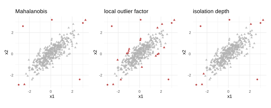
Figure 8.62: three detectors on the same contaminated data
The triangles are the five points we injected, and the red colour marks what each method flagged. The three approaches agree on the most extreme points and disagree on the borderline ones, which is the normal situation: an outlier is defined relative to a model of what is normal, and each method carries a different one.
det_tab <- data.frame(
  method = c("Mahalanobis", "local outlier factor", "isolation depth"),
  flagged = c(sum(outd$maha), sum(outd$lof), sum(outd$iso)),
  true_anomalies_found = c(sum(outd$maha & outd$truth == "anomaly"),
                           sum(outd$lof  & outd$truth == "anomaly"),
                           sum(outd$iso  & outd$truth == "anomaly")),
  false_alarms = c(sum(outd$maha & outd$truth == "normal"),
                   sum(outd$lof  & outd$truth == "normal"),
                   sum(outd$iso  & outd$truth == "normal"))
)| method | flagged | true_anomalies_found | false_alarms |
|---|---|---|---|
| Mahalanobis | 7 | 5 | 2 |
| local outlier factor | 22 | 5 | 17 |
| isolation depth | 9 | 5 | 4 |
No detector should be trusted blindly. Flagging a point is a statistical statement, never a verdict: the decision to correct it, to remove it or to study it belongs to whoever knows what the data mean. A point that is extreme because it is interesting and a point that is extreme because someone typed an extra zero look exactly the same to every algorithm of this section.