2.2 Estimation methods

To clearly understand the reason behind the multiple estimation methods, We restrict our analysis in the case of the simple linear relation.

Based on the fact that the random sample usually captures the main aspects of the DGP, so any sample moment would not differ so much from its corresponding moment in the DGP. But to infer the true relationship in the DGP, we need first to discover this relation in the sample. Remember that the point coordinates are the explanatory variable values and the dependent variable values, So if all the points lie on the same line, then the relationship will be perfect (that is, the explanatory variable is the sole factor that affects the dependent variable). Consequently, we do not need any estimation method, taking any two points to determine the line parameters. Unfortunately, for all economic processes, this case will never happen.

Specifying a line to fit points depends on the estimation method used by some criterion such as the MSE discussed above.

2.2.1 Ordinary Least Squares (OLS)

Suppose that the true DGP linear model is given by:

\[\begin{equation} Y_t=\beta_0+\beta_1X_t+\varepsilon_t \tag{2.2} \end{equation}\]

Where all the parameters and the random variable $\varepsilon_t$ are unknown.

And that the red line in the following plot is the best line by means of OLS that fits the sample points. (The source code)

#> Warning in fortify(data, ...): Arguments in `...` must be used.
#> ✖ Problematic argument:
#> • na.rm = TRUE
#> ℹ Did you misspell an argument name?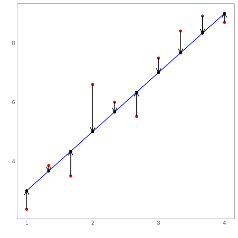

Figure 2.2: Observations vs fitted values

In this plot, for the same x-value, we have two values for the dependent variable, That of the red point, which is the true value $y_t$, and the black point that lies in the blue line along the black arrow called the fitted value $\widehat y_t$. The difference between these two values called the error of estimation given by:

\[\begin{equation} e_t=y_t-\widehat y_t \tag{2.3} \end{equation}\]

The errors also called deviations and residuals.

Even the DGP does characterize a simple linear relation between two variables, that relation can not be precisely linear so that the true model is not an exact line, that is why the model $Y_t=\beta_0+\beta_1X_t$ includes a random variable $\varepsilon_t$. That randomness included is the reason behind the existing variety of estimation methods, where each of which

It is logical to admit that the best line is the one that produces the smallest sum of the differences between observed values and fitted values, that is minimizing:

\[\begin{equation*} S(\beta_0, \beta_1)=Min\sum\limits_{t=1}^ne_t \end{equation*}\]

But this sum with this formula is not helpful because there are negative and positive errors, so many of which may cancel each other, and then many observations will have no effect on the search of the best line. However, one can suggest using the absolute value in the above sum, that is minimizing:

\[\begin{equation*} S_{abs}(\beta_0, \beta_1)=Min\sum\limits_{t=1}^n\lvert e_t\rvert \end{equation*}\]

This formula indeed save observations, but it is less convenient and not easy to be manipulated, that is why the best convenient one is the sum squared of errors:

\[\begin{equation} S(\beta_0, \beta_1)=Min\sum\limits_{t=1}^ne_t^2 \tag{2.4} \end{equation}\]

Now this principle will be used in the true model (2.2), by minimizing the corresponding errors $\varepsilon_t$ of the DGP, and this is the OLS criterion that is minimizing this sum:

\[\begin{equation} \begin{split} S(\beta_0, \beta_1)&=Min\sum\limits_{t=1}^n\varepsilon_t^2\\ & = Min\sum\limits_{t=1}^n(Y_t-\beta_0-\beta_1X_t)^2 \end{split} \tag{2.5} \end{equation}\]

The $S$ function is called The objective function.

To be not confused with the usual mathematical notations, Here we treat $(Y_t, X_t)$ as parameters because they are supposed to be known (from the sample), and the parameters $\beta_0$ and $\beta_1$ as unknown variables so that $S(\beta_0, \beta_1)$ is a function of $\beta_0$ and $\beta_1$.

we know that a function of one variable riches its optimum (maximum or minimum) when its derivative with respect to this variable equals to zero. Similarly, if this function has two variables, such as our case, then the two derivatives must be equal to zero simultaneously as follows:

\[\begin{equation*} \begin{cases} \frac{\partial S}{\partial\beta_0}&=0\\ \frac{\partial S}{\partial\beta_1}&=0 \end{cases} \end{equation*}\]

\[\begin{equation*} \begin{cases} \sum2(Y_t-\widehat\beta_0-\widehat\beta_1X_t)(-1)=0\\ \sum2(Y_t-\widehat\beta_0-\widehat\beta_1X_t)(-X_t)=0 \end{cases} \end{equation*}\]

\[\begin{equation} \begin{cases} \sum(Y_t-\widehat\beta_0-\widehat\beta_1X_t)=0\\ \sum(Y_t-\widehat\beta_0-\widehat\beta_1X_t)(X_t)=0 \end{cases} \tag{2.6} \end{equation}\]

Notice that the parameters $\beta_0$ and $\beta_1$ were replaced by the so-called estimators $\widehat\beta_0$ and $\widehat\beta_1$ respectively. As said before, they are just estimators of the true model parameters, and their accuracies depend on the chosen estimation method, among other requirements such as the sample size, etc.

From now on, we put the hat symbol on top of each OLS estimator distinguish from any other estimators ($\widehat\beta_0$, $\widehat\beta_1$ ).

Before solving these equations, it is critical to know the different notations between the true model (of the DGP) and the OLS estimated model of the sample so:

The true model:

\[\begin{equation} Y_t=\beta_0+\beta_1X_t+\varepsilon_t \tag{2.7} \end{equation}\]

The estimated model:

\[\begin{equation} Y_t=\widehat\beta_0+\widehat\beta_1X_t+e_t \tag{2.8} \end{equation}\]

The residual term:

\[\begin{equation*} e_t=Y_t-\widehat Y_t \end{equation*}\]

The fitted values:

\[\begin{equation} \widehat Y_t=\widehat \beta_0+\widehat \beta_1X_t \tag{2.9} \end{equation}\]

Using the above equations, the expression, (2.6), can be rewritten as:

\[\begin{equation} \begin{cases} \sum(Y_t-\widehat\beta_0-\widehat\beta_1X_t)=0\\ \sum(Y_t-\widehat\beta_0-\widehat\beta_1X_t)(X_t)=0 \end{cases} \implies \begin{cases} \sum e_t=0\\ \sum e_tX_t=0 \end{cases} \tag{2.10} \end{equation}\]

These two equations are called the normal equations (this term refers to the normal distribution) and hold the most critical OLS statistical properties. The first equation means that the sum of errors is always equal to zero, regardless of the used sample, and hence the mean of errors is zero:

Proof. $\sum e_t=0 \implies n\frac{\sum e_t}{n}=0 \implies \overline e=0$

While the second equation shows the linear independence between the error term $e_t$ and the explanatory $X_t$:

Proof. \[\begin{equation*} \begin{split} cov(e_t, X_t)&=E(e_t-\overline e)(X_t-\overline X)\\ &=Ee_t(X_t-\overline X)\\ &=E(e_tX_t)-E(e_t\overline X)\\ &=E(e_tX_t)-E\left(e_t\frac{\sum X_t}{n}\right)\\ &=E(e_tX_t)-\frac{1}{n}E\left(e_t\sum X_t\right)\\ &=E(e_tX_t)-\frac{1}{n}nE\sum \left(e_tX_t\right)\\ &=0 \end{split} \end{equation*}\]

Definition 2.4 The normal density function with mean $\mu$ and variance $\sigma^2$ is given by:

$f(X)=\frac{1}{\sigma\sqrt{2\pi}}e^{-\frac{1}{\sigma^2}\left(X-\mu\right)^2}whereX\sim\mathbb N(\mu, \sigma^2)$

The standard normal distribution has $\mu=0$, $\sigma^2=1$, and is given by:

$\phi(X)=\frac{1}{\sqrt{2\pi}}e^{-\frac{1}{2}\left(X\right)^2}whereX\sim\mathbb N(0,1)$

if $X\sim\mathbb N(\mu, \sigma^2) \implies\left(\frac{X-\mu}{\sigma}\right)\to X\sim\mathbb N(0,1)$

Now the solution of (2.10) is:

\[\begin{equation*} \begin{cases} \sum \left(Y_t-\widehat \beta_0-\widehat \beta_1X_t\right)=0\\ \sum \left(Y_t-\widehat \beta_0-\widehat \beta_1X_t\right)X_t=0 \end{cases} \end{equation*}\]

\[\begin{equation*} \implies \begin{cases} \sum Y_t-n\widehat \beta_0-\widehat \beta_1\sum X_t=0\\ \sum {Y_tX_t}-\widehat \beta_0\sum X_t-\widehat \beta_1\sum X_t^2=0 \end{cases} \end{equation*}\]

\[\begin{equation} \widehat \beta_0=\overline Y-\widehat \beta_1\overline X \tag{2.11} \end{equation}\]

\[\begin{equation} \widehat \beta_1=\frac{\sum {Y_tX_t}-n\overline X\overline Y}{\sum X_t^2-n\overline X^2}=\frac{\sum {(Y_t-\overline Y_t)(X_t-\overline X)}}{\sum (X_t-\overline X)^2} \tag{2.12} \end{equation}\]

provided that $\sum (X_t-\overline X)^2\neq 0$

$\widehat \beta_0$ and $\widehat \beta_1$ are called estimators of the true parameters $\beta_0$ and $\beta_1$ respectively

The expression, $\sum (X_t-\overline X)^2\neq 0$, means that it should exist some variation in the explanatory variable to allow the computation of the slope $\widehat \beta_1$. Of course, if the explanatory variable is constant, then any change that may happen in the dependent variable would be resulted by other variables than this one.

Setting the derivatives to zero can yield either a minimum or a maximum value for the objective function ($S$ in our case). To know which one we have, we use the matrix of the second derivatives, known as The Hessian matrix, so that if it is positive definite, then the objective function value is minimum. Otherwise, it is maximum.

The Hessian matrix of the OLS objective function is:

\[\begin{equation*} H(\widehat \beta_1, \widehat \beta_0)= \begin{pmatrix} \frac{\partial^2S}{\partial\widehat \beta_1^2}&\frac{\partial^2S}{\partial\widehat \beta_1\partial\widehat \beta_0}\\ \frac{\partial^2S}{\partial\widehat \beta_0\partial\widehat \beta_1}&\frac{\partial^2S}{\partial\widehat \beta_0^2} \end{pmatrix}= \begin{pmatrix} 2n&2\sum X_t\\ 2 \sum X_t&2\sum X_t^2 \end{pmatrix} \end{equation*}\]

and its determinant is:

\[\begin{equation*} \begin{split} 4n\sum X_t^2-4(\sum X_t)^2&=4n\sum X_t^2-4(n\overline X)^2\\ &=4n\sum(X_t-\overline X)^2>0 \end{split} \end{equation*}\]

Since the determinant is positive, then we have a minimum value for the OLS objective function.

2.2.1.1 Statistical properties of OLS estimators

As mentioned before, The desirable properties of any estimator are unbiasedness and efficiency. To verify these properties, we have to compute the two first moments of the estimator distribution, the mean and the variance.

Definition 2.5 The moment of order $r$ of a random variable $X$ that has the density function $f$ is given by:

$m_r=E(X^r)=\int \limits_{-\infty}^{+\infty}X^rf(X)dX$

The mean and the variance can be computed by using only the first two moments as follows:

$E(X)=E(X)=m_1$.
$V(X)=E[X-E(X)]^2=E(X^2)-[E(X)]^2=m_2-m_1^2$

The mean of $\hat \beta_1$:

We start from the true model (2.7) by taking the sum and dividing by n we get:

\[\begin{equation*} \overline Y=\beta_0+\beta_1\overline X+\overline \varepsilon....(b) \end{equation*}\]

Subtracting $(b)$ from $(a)$:

\[\begin{equation*} (Y_t-\overline Y)=\beta_1(X_t-\overline X)+(\varepsilon_t-\overline \varepsilon) \end{equation*}\]

Multiplying the equation by $\frac{(X_t-\overline X)}{\sum (X_t-\overline X)^2}$, then including the $\sum$:

\[\begin{equation*} \frac{\sum (Y_t-\overline Y)(X_t-\overline X)}{\sum (X_t-\overline X)^2}=\beta_1\frac{\sum (X_t-\overline X)^2}{\sum (X_t-\overline X)^2}+\frac{\sum (X_t-\overline X)(\varepsilon_t-\overline \varepsilon)}{\sum (X_t-\overline X)^2} \end{equation*}\]

Using (2.12) and explicit the second member of the right-hand side in more detail:

\[\begin{equation*} \widehat\beta_1=\beta_1+\frac{\sum (X_t-\overline X)\varepsilon_t}{\sum (X_t-\overline X)^2}-\frac{\overline\varepsilon\sum (X_t-\overline X)}{\sum (X_t-\overline X)^2} \end{equation*}\]

Using the arithmetic mean property $\sum (X_t-\overline X)=0$, the last formula will be:

\[\begin{equation} \widehat\beta_1=\beta_1+\frac{\sum (X_t-\overline X)\varepsilon_t}{\sum (X_t-\overline X)^2} \tag{2.13} \end{equation}\]

and hence the mean will be:

\[\begin{equation*} E(\widehat\beta_1)=\beta_1+E\left(\frac{\sum (X_t-\overline X)\varepsilon_t}{\sum (X_t-\overline X)^2}\right) \end{equation*}\]

Notice that $E(\beta_1)=\beta_1$ because it is unknown but fixed (not random).

This estimator is unbiased if the second member of the right hand side of the above formula is equal to zero.

From what has been discussed since the beginning of this book, the basic idea of econometrics is investigating all possible ways to obtain the best model that captures the main aspects of an economic process neglecting all the embarrassing marginal effects. Therefore, certain assumptions should be made to help for treating the above expression.

Using properties of the expectation, the expectation operator can be limited to $\varepsilon_t$ if the expression $(X_t-\overline X)$ can be treated as fixed, that is the regressor is not considered as a random variable, then the above equation becomes:

\[\begin{equation} E(\widehat\beta_1)=\beta_1+\frac{\sum (X_t-\overline X)E(\varepsilon_t)}{\sum (X_t-\overline X)^2} \tag{2.14} \end{equation}\]

That is the first assumption of the OLS method, which is required to ensure the unbiasedness of the estimator. For instance, the product price is exactly determined by the firm if used in a model that predicts sales. Or the effect of the number of working hours on productivity, etc. However, There exist also many other cases where the regressor is a random variable that will be treated further in this book.

Definition 2.6 If $X$ and $Y$ are random variables with the density function $f$ then:

$E(X)=\int \limits_{-\infty}^{+\infty}Xf(X)dX$
$E(\alpha X)=\alpha E(X)$
$E(\alpha X+\beta Y)=\alpha E(X)+\alpha E(Y)$

Where $\alpha$ and $\beta$ are constant terms.

And if $X$ and $Y$ are independent of each other then:

$E(XY)=E(X)E(Y)$

The previous assumption alone is not sufficient to get the unbiasedness since the expression that contains the regressor is not equal to zero. To be equal to zero, however, we have to assume that the errors mean zero $E(\varepsilon_t)=0$.

It is nearly impossible for the dependent variable of the true model (2.7) to be only affected by a single regressor $X_t$. So it must exist other minor effects from other unknown variables grouped in a single random variable $\varepsilon_t$. These marginal factors should likely affect positively and negatively the model such that, in total, the effects cancel each other. Otherwise, the model parameters will change, which is in contradiction with the fact that this model is true. Statistically, this assumption is expressed by $E(\varepsilon_t)=0$. That is the second assumption of the OLS method.

The mean of $\widehat \beta_0$:

Using the true model (2.7) and the estimated model (2.8) as follows:

\[\begin{equation*} \begin{cases} Y_t=\beta_0+\beta_1X_t+\varepsilon_t\\ Y_t=\widehat \beta_0+\widehat \beta_1X_t+e_t \end{cases} \implies \begin{cases} \overline Y=\beta_0+\beta_1\overline X+\overline \varepsilon\\ \overline Y=\widehat \beta_0+\widehat \beta_1\overline X+(\overline e=0) \end{cases} \end{equation*}\]

Then by subtracting the second equation from the first one we obtain:

\[\begin{equation} \widehat \beta_0=\beta_0-(\widehat \beta_1-\beta_1)\overline X+\overline \varepsilon \tag{2.15} \end{equation}\]

Including then the expectation operator, the last formula will be:

\[\begin{equation*} E(\widehat \beta_0)=\beta_0-\overline XE(\widehat \beta_1-\beta_1)+E(\overline \varepsilon) \end{equation*}\]

The last two members of the right hand side $E(\widehat \beta_1-\beta_1)$ and $E(\overline \varepsilon)=0$, both of which are equal to zero because:

\[\begin{equation*} E(\overline \varepsilon)=E\left(\frac{\sum \varepsilon_t}{n}\right)=\sum \left(\frac{E(\varepsilon_t)}{n}\right)=0 \end{equation*}\]

\[\begin{equation*} E(\widehat \beta_1-\beta_1)=E(\widehat \beta_1)-\beta_1=\beta_1-\beta_1=0 \end{equation*}\]

Finally:

\[\begin{equation*} E(\widehat \beta_0)=\beta_0 \end{equation*}\]

In the simple linear regression, unbiasedness of the OLS estimators requires only two assumptions:

Assumption 1: The regressors should be fixed.
Assumption 2: The mean of the error term should be equal to zero.

The variance of $\widehat \beta_1$:

Using the expression (2.13), the variance is given by:

\[\begin{equation*} V(\widehat \beta_1)=E\left(\widehat \beta_1-E(\hat \beta_1)\right)^2=E\left(\widehat \beta_1-\beta_1\right)^2=E\left(\frac{\sum (X_t-\overline X)\varepsilon_t}{\sum (X_t-\overline X)^2}\right) \end{equation*}\]

Since the regressor is not random, we can simplify this expression by substituting $\frac{(X_t-\overline X)}{\sum (X_t-\overline X)^2}$ by a single fixed variable $W_t$ and using the statistical properties of the variance, then will have:

\[\begin{equation*} \begin{split} V(\widehat \beta_1)&=E\left(\sum W_t\varepsilon_t\right)^2\\ &=E\left(\sum W_t^2\varepsilon_t^2+2\sum \limits_t\sum \limits_sW_tW_s\varepsilon_t\varepsilon_s\right) \end{split} \end{equation*}\]

Using the assumption 1 with the non random variable $W_t$ we obtain:

$V(\widehat \beta_1)=\sum W_t^2E(\varepsilon_t^2)+2\sum \limits_t\sum \limits_sW_tW_sE(\varepsilon_t\varepsilon_s)$ where $t<s$.

And by using the assumption 2, the variance and the covariance of the error term will be:

\[\begin{equation*} V(\varepsilon_t)=E\left( \varepsilon_t-E(\varepsilon_t)\right)^2=E(\varepsilon_t^2) \end{equation*}\]

\[\begin{equation*} cov(\varepsilon_t,\varepsilon_s)=E\{\left(\varepsilon_t-E(\varepsilon_t)\right)\left(\varepsilon_s-E(\varepsilon_s)\right)\}=E(\varepsilon_t\varepsilon_s) \end{equation*}\]

Definition 2.7 If $X$ and $Y$ are random variabels with the density function $f$, then:

$V(X)=E\left(X-E(X)\right)^2=\int \limits_{-\infty}^{+\infty}\left(X-E(X)\right)^2f(X)dX$
$V(\alpha X)= \alpha^2V(X)$

Where $\alpha$ and $\beta$ are constant terms.

$V(\alpha X+\beta Y)= \alpha^2V(X)+\beta^2V(Y)+2\alpha \beta cov(X,Y$

The first member on the right-hand side represents the variance of the random term, which is the volatility around the line of the DGP model. Intuitively, the volatility of the deviations has to be constant among the individuals in sectional data or overtime in time series. The reason is that the true model fits all the data similarly because it is supposed to catch the main aspects for all the individuals or at least most of them. That is, the neglected variables grouped in the error term would likely affect all the individuals. If the volatility is large for some individuals, then these individuals may be exposed to strong effects from variables that were supposed neglected. Therefore, we assume that the error variance is constant, and that is the assumption 3, that is expressed by:

\[\begin{equation*} E(\varepsilon_t^2)=\sigma^2 \end{equation*}\]

without the index $t$ to mean constant.

From the DGP model $Y_t=\beta_0+\beta_1 X_t+\varepsilon_t$, the quantity $\beta_0+\beta_1 X_t$ is considered as non random. By using then the statistical properties of the variance, we will have $V(Y_t)=V(\varepsilon_t)=E(\varepsilon_t^2)=\sigma^2$, that is the dependent variable, and the error term of the DGP have the same variance. That is consistent with the explanation discussed earlier so that the only source of randomness in the dependent variable is the error term.

For the second member, let us suppose there exists a strong correlation between two different disturbances, say $t$ and $s$. That correlation implies dependence between the corresponding individuals $Y_t$ and $Y_s$, means that at least one of which, say $t$, (depending on the direction of causality) is affected not just by the single explanatory variable $X_t$, but also by the other individual $s$. Therefore, $Y_s$ must be taken into account in the model as an additional effect. But since the theoretical model has only one regressor $X_t$, we can admit as an assumption that no correlation between any two different disturbances. We have thus the assumption 4:

\[\begin{equation*} E(\varepsilon_t\varepsilon_s)=0 \end{equation*}\]

Finally, we obtain the variance expression:

\[\begin{equation*} V(\widehat \beta_1)=\sum W_t^2\sigma^2)=\sigma^2\left(\frac{\sum (X_t-\overline X)^2}{\left[\sum (X_t-\overline X)^2\right]^2}\right) \end{equation*}\]

And hence:

\[\begin{equation} V(\widehat \beta_1)=\frac{\sigma^2}{\sum (X_t-\overline X)^2} \tag{2.16} \end{equation}\]

The variance of $\widehat \beta_0$:

Using (2.15)

\[\begin{equation*} \begin{split} V(\widehat \beta_0)&=E(\widehat \beta_0-\beta)^2\\ &=E\left(\overline \varepsilon-(\widehat \beta_1-\beta_1)\overline X\right)^2\\ &=E\left(\overline \varepsilon^2-2\overline X(\widehat \beta_1-\beta_1)\overline \varepsilon+\overline X^2(\widehat \beta_1-\beta_1)^2\right) \end{split} \end{equation*}\]

Let us take each member of the right-hand side separately. Using assumptions 3 and 4, the first member will be:

\[\begin{equation*} \begin{split} E(\overline \varepsilon)&=E\left(\frac{\left(\sum \varepsilon_t\right)^2}{n^2}\right)\\ &=\frac{1}{n^2}E\left(\sum \varepsilon_t^2+2\sum \limits_{t<s}\sum \limits_s\varepsilon_t\varepsilon_s \right)\\ &=\frac{1}{n^2}\sum E(\varepsilon_t^2)\\ &=\frac{n\sigma^2}{n^2}\\ &=\frac{\sigma^2}{n} \end{split} \end{equation*}\]

Using assumptions 1,3 and 4 and the following result:

\[\begin{equation*} \begin{split} E\left((\widehat \beta_1-\beta_1)\overline \varepsilon\right)&=E \left((\sum W_t\varepsilon_t)\left(\frac{\sum \varepsilon_t}{n}\right)\right)\\ &=\frac{1}{n}E\left(\sum W_t\varepsilon_t^2+\sum \limits_{t<s}\sum \limits_s W_t\varepsilon_t\varepsilon_s\right)\\ &=\frac{1}{n}\left(\sum W_tE(\varepsilon_t^2)+\sum \limits_{t<s}\sum \limits_s W_tE(\varepsilon_t\varepsilon_s)\right)\\ &=\frac{1}{n}\left(\sigma^2\sum W_t+\sum \limits_{t<s}\sum \limits_s W_tE(\varepsilon_t\varepsilon_s)\right)\\ &=0 \end{split} \end{equation*}\]

Since the third member contains the variance of $\widehat \beta_1$ that has been already computed, then the variance of $\widehat \beta_0$ will be:

\[\begin{equation} V(\widehat \beta_0)=\sigma^2\left(\frac{1}{n}+\frac{\overline X^2}{\sum (X_t-\overline X)^2}\right) \tag{2.17} \end{equation}\]

The covariance of $(\widehat \beta_1, \widehat \beta_0)$:

Using (2.15) and the above results, this covariance will be:

\[\begin{equation*} \begin{split} cov(\widehat \beta_1, \widehat \beta_0)&=E\left[(\widehat \beta_1-\beta_1)(\widehat \beta_0-\beta_0)\right]\\ &=E\left[(\widehat \beta_1-\beta_1)\left(\overline \varepsilon-(\widehat \beta_0-\beta_0)\overline X\right)\right]\\ &=E\left[(\widehat \beta_1-\beta_1)\overline \varepsilon\right]-\overline XE(\widehat \beta_1-\beta_1)^2\\ &=-\bar XE(\widehat \beta_1-\beta_1)^2 \end{split} \end{equation*}\]

\[\begin{equation} cov(\widehat \beta_1, \widehat \beta_0)=\frac{-\sigma^2\overline X^2}{\sum (X_t-\overline X)} \tag{2.18} \end{equation}\]

The variances and the covariance computed above can be summarized in one symmetric matrix called The variance matrix as follows:

\[\begin{equation} Var(\widehat \beta_1, \widehat \beta_0) \begin{pmatrix} V(\widehat \beta_1)&cov(\widehat \beta_1, \widehat \beta_0)\\ cov(\widehat \beta_1, \widehat \beta_0)&V(\widehat \beta_0) \end{pmatrix} \tag{2.19} \end{equation}\]

To be constant and finite, the variance matrix of the OLS estimators in the simple linear regression requires the following assumptions:

Assumption 1: the regressor is not random.
Assumption 3: the variance of the error term is constant $E(\varepsilon_t^2)=\sigma^2$.
Assumption 4: no correlation between error terms $E(\varepsilon_t\varepsilon_s)=0$.

Estimation of $\sigma^2$:

The variance matrix can not be computed, since it contains the quantity $\sigma^2$ that is unknown. Thus we have to estimate this quantity as we did with the other model parameters by making use of the sample at hand. The first estimator that comes in mind is the sample variance of errors $\sigma_e^2=\frac{\sum e_t^2}{n}$, which can be computed easily from the observations, but if it is at least unbiased. Let us start with the estimated model (2.8):

\[\begin{equation*} Y_t=\widehat Y_t+e_t\implies\frac{\sum Y_t}{n}=\frac{\sum \hat Y_t}{n}+\frac{\sum e_t}{n}\implies \overline Y=\overline {\widehat Y}+\overline e \end{equation*}\]

Using $\sum e_t=0$ from the normal equations (2.10), the last expression gives:

\[\begin{equation*} \overline Y=\overline {\widehat Y} \end{equation*}\]

The equality of the sample mean $\bar Y$ and the fitted mean $\bar {\hat Y}$ computed by OLS is an important property so that it will be used to compare the fitted values to the observations.

Using the result $\overline Y=\overline {\widehat Y}$, the residual $e_t$ is given by:

\[\begin{equation*} e_t=Y_t-\widehat Y_t=Y_t-\overline Y+\overline {\widehat Y}-\widehat Y_t=(Y_t-\overline Y)+(\overline {\widehat Y}-\widehat Y_t) \end{equation*}\]

The first member of the right hand side can be derived from the true mode (2.7) as follows:

\[\begin{equation*} Y_t-\overline Y_t=\beta_1(X_t-\overline X)+(\varepsilon_t-\overline \varepsilon) \end{equation*}\]

Similarly, by using the estimated model (2.8) the last member will be:

\[\begin{equation*} \overline {\widehat Y}-\widehat Y=\widehat \beta_0+\widehat \beta_1\overline X-\widehat \beta_0-\widehat \beta_1X_t=-\widehat \beta_1(X_t-\overline X) \end{equation*}\]

Substituting the two last expressions into the above formula of $e_t$, we obtain:

\[\begin{align} e_t&=\beta_1(X_t-\overline X)+(\varepsilon_t-\overline \varepsilon)-\widehat \beta_1(X_t-\overline X) \notag\\ &=(\varepsilon_t-\overline \varepsilon)-(\widehat \beta_1-\beta_1)(X_t-\overline X) \tag{2.20} \end{align}\]

Then by squaring and summing, we obtain:

\[\begin{equation*} \begin{split} \sum e_t^2&=\sum \left[(\varepsilon_t-\overline \varepsilon)-(\widehat \beta_1-\beta_1)(X_t-\overline X)\right]^2\\ &=\sum (\varepsilon_t-\overline \varepsilon)^2-2(\widehat \beta_1-\beta_1)\sum (X_t-\overline X)(\varepsilon_t-\overline \varepsilon)+(\widehat \beta_1-\beta_1)^2\sum (X_t-\overline X)^2 \end{split} \end{equation*}\]

Notice that:

\[\begin{equation*} \begin{split} \sum (X_t-\overline X)(\varepsilon_t-\overline \varepsilon)&=\sum (X_t-\overline X)\varepsilon_t-\sum (X_t-\overline X)\overline \varepsilon)\\ &=\sum (X_t-\overline X)(\varepsilon_t-\overline \varepsilon)\\ &=\sum (X_t-\overline X)\varepsilon_t-\overline \varepsilon\underbrace{\sum (X_t-\overline X))}_{=0}\\ &=\sum (X_t-\overline X)\varepsilon_t \end{split} \end{equation*}\]

Using this result to substitute the expression (2.13) into the above formula as follows:

\[\begin{equation*} \begin{split} \sum e_t^2&=\sum (\varepsilon_t-\overline \varepsilon)^2-2(\widehat \beta_1-\beta_1)^2\sum (X_t-\overline X)^2+(\widehat \beta_1-\beta_1)^2\sum (X_t-\overline X)^2\\ &=\sum (\varepsilon_t-\overline \varepsilon)^2-(\widehat \beta_1-\beta_1)^2\sum (X_t-\overline X)^2 \end{split} \end{equation*}\]

Including the expectation operator:

\[\begin{equation} E\left(\sum e_t^2\right)=E\left(\sum (\varepsilon_t-\overline \varepsilon)^2\right)-E\left((\widehat \beta_1-\beta_1)^2\right)\sum (X_t-\overline X)^2 \tag{2.21} \end{equation}\]

For simplicity, we will develop each member of the right-hand side separately. So starting with the first member:

\[\begin{equation*} \begin{split} E\left[\sum (\varepsilon_t-\overline \varepsilon)^2\right]&=E\left[\sum (\varepsilon_t^2-2\varepsilon_t\overline \varepsilon+\overline \varepsilon^2)\right]\\ &=E\left(\sum \varepsilon_t^2-2\overline \varepsilon\sum \varepsilon_t+n\overline \varepsilon^2\right)\\ &=E\left(\sum \varepsilon_t^2-n\overline \varepsilon^2\right)\\ &=\sum E(\varepsilon_t^2)-nE(\overline \varepsilon^2)\\ &=\sum E(\varepsilon_t^2)-nE\left( \frac{\sum \varepsilon_t}{n}\right)^2\\ &=\sum E(\varepsilon_t^2)-n\frac{1}{n^2}E\left(\sum \varepsilon_t^2+2\sum \limits_{t<s}\sum \limits_s\varepsilon_t\varepsilon_s\right)\\ &=\sum E(\varepsilon_t^2)-\frac{1}{n}\left(\sum \underbrace{E(\varepsilon_t^2)}_{\sigma^2}+2\sum \limits_{t<s}\sum \limits_s\underbrace{E(\varepsilon_t\varepsilon_s)}_{=0}\right)\\ &=n\sigma^2-\frac{1}{n}n\sigma^2\\ &=(n-1)\sigma^2 \end{split} \end{equation*}\]

And for the second member we have:

\[\begin{equation*} \begin{split} E\left[(\widehat \beta_1-\beta_1)\right]\sum (X_t-\overline X)^2&=\frac{\sigma^2}{\sum (X_t-\overline X)^2}\sum (X_t-\overline X)^2\\ &=\sigma^2 \end{split} \end{equation*}\]

Substituting these results in the main equation above, we obtain:

\[\begin{equation*} \begin{split} E(\sum e_t^2)&=(n-1)\sigma^2-\sigma^2\\ &=(n-2)\sigma^2 \end{split} \end{equation*}\]

Now let us verify the unbiasedness of the sample variance:

\[\begin{equation*} E\left(\frac{\sum e_t^2}{n}\right)=\frac{(n-2)\sigma^2}{n}\implies E(\sigma_e^2)=\frac{(n-2)\sigma^2}{n}\neq \sigma^2 \end{equation*}\]

Unexpectedly, this result indicates that the error variance of the sample is not unbiased. However, it can be used for the derivation of an unbiased one as follows:

\[\begin{equation*} E\left(\sum e_t^2\right)=(n-2)\sigma^2\implies E\left(\frac{\sum e_t^2}{n-2}\right)=\sigma^2 \end{equation*}\]

Finally, we obtained an unbiased estimator for the unknown variance denoted by $s^2$:

\[\begin{equation} s^2=\frac{\sum e_t^2}{n-2} \tag{2.22} \end{equation}\]

The square root of this variance is called The standard error of regression.

All the above quantities now can be computed after replacing the theoretical variance $\sigma^2$ by $s^2$.

The unbiasedness of this estimator requires assumptions 1,3,4.

In practice, we do not have to compute the different parameters, since there exist many software tools that can do everything for us. Throughout this book, I will be using the powerful open source programming language R.

Example 2.1 For the sake of clarity, we use 100 simulated data where the dependent variable is related to the explanatory variable by the true relation $Y_t=10+4X_t+\varepsilon_t$. Then we take out 20 samples from this population and apply OLS regression.

In R:

In R the lm function (linear models) applies the OLS regression method.

# This library is a collection of packages 
# for data manipulation and plotting.
library(tidyverse)
# keep the result reproducible
set.seed(3)
# draw the error term from the standard 
# normal distribution
epsilon <- rnorm(100)
# Draw the regressor from the normal distribution
# with mean 10 and standard deviation 5
set.seed(1)
x <- rnorm(100, 10, 5)
# assume that this is the true model
y <- 10 + 4 * x + epsilon
# put the variables in a data frame object for 
# easy manipulation named "df" (you can put any name you want)
df <- tibble(y, x)
# take out randomly a 20 samples from the true model
df1 <- df[sample(NROW(df), 20), ]
# estimate the model and store it in the name "model_ols"
# (you can choose other name)
model_ols <- lm(y ~ x, data = df1)
# display the results using the broom function tidy
tidy(model_ols)

Table 2.1: the results of estimation
term	estimate	std.error	statistic	p.value
(Intercept)	9.261277	0.5820879	15.91044	0
x	4.054895	0.0536795	75.53904	0

In Python:

First of all, to be able to use python in Rmarkdown, we have to call the R package reticulate before any python code. Then we can start by calling the most important python packages, the numpy package for mathematical functions and generating random samples, and other functionalities, the pandas for data manipulations, statsmodels for econometrics and time series analysis, and mathplotlib and seaborn for visualization.

import numpy as np
import pandas as pd
import statsmodels.api as sm
# Set the seed for reproducible results
np.random.seed(3)
# Generate 100 standard normal values for 
# the error variable
epsilonP = np.random.normal(0,1,100)
# Generate 100 values from the normal distribution
# with mean 10 and std 4
np.random.seed(1)
xP = np.random.normal(loc=10, scale=5, size=100)
# Specify the relationship of the DGP model
yP = 10 + 4 * xP + epsilonP
# Put the variables in a data frame
dfP = pd.DataFrame({'yP':yP,'xP': xP})
# Take out a sample of 20 observations
dfP1 = dfP.sample(n=20)
# Define the dependent variable and the regressor 
Y = dfP1['yP']
X = dfP1['xP']
# By default the model does not include a constant
# so we should include it manually
X = sm.add_constant(X)
# Build the OLS model
modelP = sm.OLS(Y,X)
# Fit the model 
results = modelP.fit()

# converts the resulted table into a pandas data frame
summ = results.summary2().tables[1]
# display the results
summ

Table 2.2: the results of estimation
	Coef.	Std.Err.	t	P>\|t\|	[0.025 ]
const	10.674788	0.5167838	20.6562	0	9.589066	11.760510
xP	3.919729	0.0476934	82.1860	0	3.819529	4.019929

As we can see, the OLS estimates are very close to those of the true model. Notice that, every time we increase the sample size, we should obtain more accurate estimates. For instance, if we try a larger sample size, say 70, then the new estimates will be.

In R:

set.seed(123)
df2 <- df[sample(NROW(df), 70),]
model2 <- lm(y~x, data=df2)
tidy(model2)

Table 2.3: the results of estimation
term	estimate	std.error	statistic	p.value
(Intercept)	10.261210	0.2536604	40.45255	0
x	3.978317	0.0218554	182.02932	0

In Python:

np.random.seed(123)
# Now take 70 samples
dfP2 = dfP.sample(n=70)
Y = dfP2['yP']
X = dfP2['xP']
X = sm.add_constant(X)
modelP2 = sm.OLS(Y,X)
results2 = modelP2.fit()
summ2 = results2.summary2().tables[1]

Table 2.4: the results of estimation
	Coef.	Std.Err.	t	P>\|t\|	[0.025 ]
const	10.313847	0.3198855	32.2423	0	9.675525	10.952168
xP	3.970234	0.0289314	137.2293	0	3.912502	4.027966

As we see, the new estimates (10.313847, 3.978317 ) are slightly closer to the true parameters (10, 4) than the old ones (9.261277 , 4.054895) with less samples.

We can use that example to check the unbiasedness of the estimator $\widehat \beta_1$ by computing the estimates from 1000 different samples as follows:

In R:

# we create a function that takes out randomly
# 20 samples from the original data
coeff  <- function(nrow) {
  # create a function that takes out randomly 30
  # samples from the original data and stored in
  # data.F object.
  data.F <- df[nrow, ]
  # estimate the model with the new sample
  model <- lm(y ~ x, data = data.F)
  # extract only the second coefficient (the slop)
  model$coefficients[[2]]
}
# generate 1000 different vector where each one
# has different set of rows sampled from the original
# data df
generated.samples <- replicate(n = 1000, sample(NROW(df), 20))
# since generated.samples is a matrix,  use  the apply
# function to apply the above coeff function to each column
result <- apply(generated.samples, 2, coeff)
# compute the mean and the standard deviation

d <- data.frame(mean = mean(result), sd = sd(result))
d

Table 2.5: the mean and the standard deviation of the simulation
mean	sd
3.995619	0.0440611

It is better to plot the histogram of the result:

# we store the result object in data frame 
# for ease of manipulation
D <- data.frame(result)

ggplot(D, aes(result)) +
    geom_histogram(
    aes(result, y = ..density..),
    color = "black",
    bins=50,
    fill = 'grey'
  ) +
  geom_density(color='red')+
  geom_vline(xintercept = mean(D$result),color = "blue",lwd = 1.2) +
  geom_vline(xintercept = 4,color = "red",lwd = 1.2) +
  geom_vline( xintercept = mean(D$result) - 2 * sd(D$result),color = "green", lwd = 1.2 ) +
  geom_vline(xintercept = mean(D$result) + 2 * sd(D$result),color = "green",lwd = 1.2 )+
  theme_classic()

#> Warning: The dot-dot notation (`..density..`) was deprecated in ggplot2 3.4.0.
#> ℹ Please use `after_stat(density)` instead.
#> This warning is displayed once per session.
#> Call `lifecycle::last_lifecycle_warnings()` to see where this warning was
#> generated.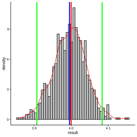

Figure 2.3: The distribution of the slop in R

As we see, all the different estimates $\widehat \beta_1$ are around the true value $\beta_1$, and the empirical mean in blue is much closer to the true value both inside the region of 95% confidence level bounded by the two green lines. The most important result, however, is that the distribution has the bell shape of the normality distribution.

We can follow the same steps as we did above to display the distribution plot of $\widehat\beta_0$ as follows:

coeff0  <- function(nrow) {
  model <- lm(y ~ x, data = df[nrow, ])
  model$coefficients[[1]]
}

result0 <- apply(generated.samples, 2, coeff0)
D0 <- data.frame(result0)

ggplot(D0, aes(result0)) +
  geom_histogram(
    aes(x=result0, y = ..density..),
    color = "black",
    bins = 50,
    fill = 'grey'
  ) +
  geom_density(color = "red") +
  geom_vline(xintercept = mean(D0$result0),
             color = "blue",
             lwd = 1.2) +
  geom_vline(xintercept = 10,
             color = "red",
             lwd = 1.2) +
  geom_vline(
    xintercept = mean(D0$result0) - 2 * sd(D0$result0),
    color = "green",
    lwd = 1.2
  ) +
  geom_vline(
    xintercept = mean(D0$result0) + 2 * sd(D0$result0),
    color = "green",
    lwd = 1.2
  ) +
  theme_classic()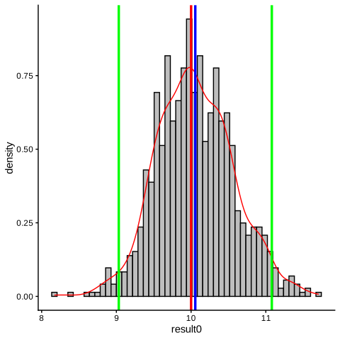

Figure 2.4: The distribution of the intercept in R

Last thing to mention is that any R object has many attributes that can be extracted using the R function attributes. we can for instance extract all the attributes by:

attributes(model_ols)

#> $names
#>  [1] "coefficients"  "residuals"     "effects"       "rank"         
#>  [5] "fitted.values" "assign"        "qr"            "df.residual"  
#>  [9] "xlevels"       "call"          "terms"         "model"        
#> 
#> $class
#> [1] "lm"

To extract a single attribute use the $ symbol.

model_ols$coefficients

#> (Intercept)           x 
#>    9.261277    4.054895

In Python:

We can do the same above steps using python. We simulate 1000 samples then we fit a model for each set.

# We create an empty object
resultsP = np.empty(shape=1000)

# We fit a model for each set
for i in np.arange(1000):
    np.random.seed(i)
    dfP_sim = dfP.sample(n=20)
    Y = dfP_sim['yP']
    X = dfP_sim['xP']
    X = sm.add_constant(X)
    model = sm.OLS(Y,X)
    fitted = model.fit()
    res = fitted.params.iloc[1,]
    resultsP[i] = res
print(np.round(resultsP.mean(),4),np.round(resultsP.std(),4))

#> 3.9932 0.0522

To visualize the results with the confidence interval, we make use of the seaborn package that uses matplotlib as a backend.


import matplotlib.pyplot  as plt
import seaborn as sns

# Create a placeholder for the figure
fig= plt.figure(figsize=(5,5))

# extract the slop and thee confidence interval bounds
slop=results.params.iloc[1,]
lower = results.conf_int().iloc[1,].iloc[0,]
upper = results.conf_int().iloc[1,].iloc[1,]

# create a density plot 
g1=sns.displot(resultsP, bins=50, kde=True)

# Cretae a vertical line
g2=plt.axvline(resultsP.mean(), 0, 12.5, color='r')
g3 = plt.axvline(lower, 0, 12.5, color='g')
g4 = plt.axvline(upper, 0, 12.5, color='g')
g5 = plt.axvline(slop, 0, 12.5, color='darkblue')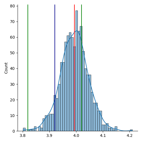

plt.show()

Figure 2.5: The distribution of the slope in python

2.2.1.2 Geometric interpretation of the OLS method

Let us take the following estimated model:

\[\begin{equation*} Y_t=\widehat \beta_0+\widehat \beta_1X_t+e_t \end{equation*}\]

with the estimated line equation:

\[\begin{equation*} \widehat Y_t=\widehat \beta_0+\widehat \beta_1X_t \end{equation*}\]

They can be rewritten in terms of vectors:

\[\begin{equation*} \overrightarrow Y=\widehat \beta_0\overrightarrow U+\widehat \beta_1\overrightarrow X+\overrightarrow e \end{equation*}\]

\[\begin{equation*} \overrightarrow {\widehat Y}=\hat \beta_0\overrightarrow U+\widehat \beta_1\overrightarrow X \end{equation*}\]

Where:

\[\begin{equation*} \overrightarrow Y= \begin{pmatrix} y_1\\ y2\\ ..\\ y_n \end{pmatrix} \quad \overrightarrow {\widehat Y}= \begin{pmatrix} \widehat y_1\\ \widehat y_2\\ ..\\ \widehat y_n \end{pmatrix} \quad \overrightarrow X= \begin{pmatrix} x_1\\ x_2\\ ..\\ x_n \end{pmatrix} \quad \overrightarrow U= \begin{pmatrix} 1\\ 1\\ ..\\ 1 \end{pmatrix} \quad \overrightarrow e= \begin{pmatrix} e_1\\ e_2\\ ..\\ e_n \end{pmatrix} \end{equation*}\]

From the second formula, we see that the vector $\overrightarrow {\widehat Y}$ is a linear combination of the two vectors $\overrightarrow U$ and $\overrightarrow X$ means that these vectors are on the same hyperplane. Whereas, the vector $\overrightarrow Y$ is in higher space because of the vector $\overrightarrow e$ (from the first formula). Since we want each fitted value to be closer to its corresponding observed one. The euclidian distance then between $\overrightarrow {\widehat Y}$ and $\overrightarrow Y$ should be at its minimum. The minimum distance between an observed point and the hyperplane that contains the fitted values is the orthogonal projection represented by the vector norm $\overrightarrow e$ in our case.

#> Warning in geom_segment(aes(x = 1, y = 1, xend = 3, yend = 8)): All aesthetics have length 1, but the data has 5 rows.
#> ℹ Please consider using `annotate()` or provide this layer with data containing
#>   a single row.

#> Warning in geom_segment(aes(x = 1, y = 1, xend = 8, yend = 1)): All aesthetics have length 1, but the data has 5 rows.
#> ℹ Please consider using `annotate()` or provide this layer with data containing
#>   a single row.

#> Warning in geom_segment(aes(x = 5, y = 8, xend = 5, yend = 3), linetype = "dashed", : All aesthetics have length 1, but the data has 5 rows.
#> ℹ Please consider using `annotate()` or provide this layer with data containing
#>   a single row.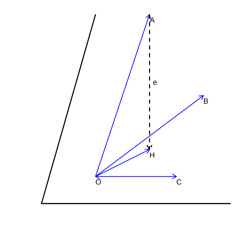

Figure 2.6: Geometric interpretaion of OLS

The vectors $\overrightarrow Y$, $\overrightarrow {\widehat Y}$, $\overrightarrow X$, $\overrightarrow U$, and $\overrightarrow e$ are represented by $\overrightarrow {OA}$, $\overrightarrow {OH}$, $\overrightarrow {OB}$, $\overrightarrow {OC}$, and $\overrightarrow {HA}$ respectively.

Formally, the OLS criterion can be expressed in terms of vectors as follows:

\[\begin{equation} Min\sum e_t^2=Min\lVert \overrightarrow e \rVert^2=Min\lVert \overrightarrow {HA} \rVert^2 \tag{2.23} \end{equation}\]

Where the notation $\lVert\quad \rVert$ indicates the length of the vector (the norm). Using the orthogonal projection rules we have:

\[\begin{align*} \begin{cases} \overrightarrow {HA}.\overrightarrow {OC}=0\\ \overrightarrow {HA}.\overrightarrow {OB}=0 \end{cases} &\implies \begin{cases} \langle Y-\widehat \beta_0-\widehat \beta_1X,U\rangle=0\\ \langle Y-\widehat \beta_0-\widehat \beta_1X,X\rangle=0 \end{cases}\\ &\implies \begin{cases} \sum Y_t-n\widehat \beta_0-\widehat \beta_1\sum X_t=0\\ \sum Y_tX_t-\widehat \beta_0\sum X_t-\widehat \beta_1\sum X_t^2=0 \end{cases} \end{align*}\]

These are the normal equations that have been obtained before with the algebraic method (2.6).

2.2.1.3 OLS regression without regressors

What happens if we consider applying the OLS method using only the constant term without any regressor terms? The answer to this question will help to understand the importance of the constant term. Using the geometric method as described in the plot below, the OLS criterion in such case will be rewritten by:

\[\begin{equation*} Min\sum e_t^2=Min\lVert CA\rVert^2 \end{equation*}\]

Now we have only the vectors $Y$ ($\overrightarrow {OA}$), $U$ ($\overrightarrow {OC}$), and $e$ ($\overrightarrow {CA}$).

#> Warning in geom_segment(aes(x = 1, y = 1, xend = 3, yend = 8)): All aesthetics have length 1, but the data has 3 rows.
#> ℹ Please consider using `annotate()` or provide this layer with data containing
#>   a single row.

#> Warning in geom_segment(aes(x = 1, y = 1, xend = 8, yend = 1)): All aesthetics have length 1, but the data has 3 rows.
#> ℹ Please consider using `annotate()` or provide this layer with data containing
#>   a single row.

#> Warning in geom_segment(aes(x = 6, y = 8, xend = 6, yend = 2), linetype = "dashed", : All aesthetics have length 1, but the data has 3 rows.
#> ℹ Please consider using `annotate()` or provide this layer with data containing
#>   a single row.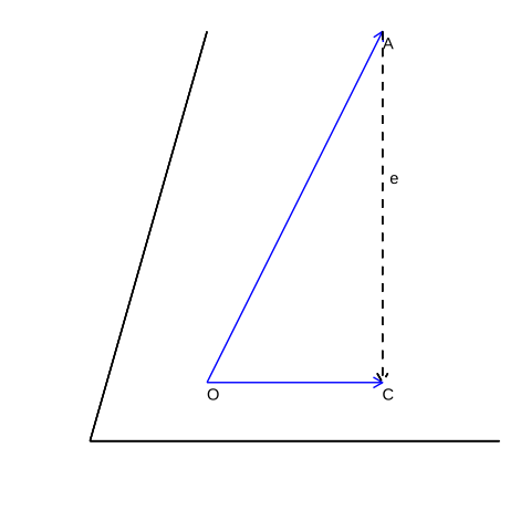

Figure 2.7: OLS regression without regressors

Using the plot, the orthogonal projection implies that:

\[\begin{equation*} \begin{split} Y_t=\widehat \beta_0+e_t&\implies\overrightarrow Y=\widehat \beta_0\overrightarrow U+\overrightarrow e\\ &\implies \langle Y-\widehat \beta_0U, U\rangle=0\\ &\implies \sum Y_t-n\widehat \beta_0=0\\ &\implies \widehat \beta_0=\frac{\sum Y_t}{n}\\ &\implies \widehat \beta_0=\overline Y\\ &\implies \overrightarrow {OC}=\overline Y \end{split} \end{equation*}\]

We conclude that the orthogonal projection on the hyperplane that contains only the constant term gives the sample mean $\overline Y$. This result is a fundamental element when further analyzing variances.

2.2.1.4 OLS assumptions

As discussed before, The OLS method requires certain assumptions to give competitive estimators:

A1: The observations are not random.

A2: The zero mean of errors $E(\varepsilon_t)=0$.

A3: The variance is constant for all sample individuals $E(\varepsilon_t^2)=\sigma^2$, and this case is called homoskedasticity. Otherwise, when it is varying over individuals, we will have a heteroskedasticity problem.

A4: The errors are uncorrelated when any two individuals are linearly independent $E(\varepsilon_t\varepsilon_s)=0$. Otherwise, we say that the errors are autocorrelated, or serially correlated.

Assumptions 2, 3, and 4 can be expressed together by $\varepsilon_t \sim IID(0\;, \sigma^2)$. Then we say that the disturbances are independently and identically distributed with zero mean and constant variance.

A5: The assumption of no correlation between the error term and the regressor is known as orthogonality condition, not treated yet because implied from the fixed regressor assumption. But it will be useful if the latter is not satisfied, and the regressors are random instead (it will be discussed further in the next chapter).

A6: This assumption was not involved in the previous analysis because not needed but required before starting the investigation, in contrast to the other assumptions used along with the investigation process. This assumption is called linearity, which means the DGP model is assumed to have a linear form. Not that the linearity is in parameters ($\beta_0\;, \beta_1$ in our case), not in regressors. For instance, the model $Y_t=\beta_0+\beta_1X_t^2$ is not linear in the regressor, but linear in parameters so that it still be treated as a linear. However, to be able to draw a line from that model, we should use the transformed regressor $X_t^2$ in the x-axis, not the original one $X_t$.

A7: You may have heard about the model parameters constancy assumption, not mentioned yet. Implied from the linearity assumption such that if the parameter values were changed at a particular point somewhere in the scatter points, then the line would suddenly change direction resulting, say in two parts, each part has a different one. So for these two parts of the scatter points, we could suggest linearly approximate each one separately, instead of approximating the whole. This assumption required more in the cases of nonlinear models.

A8: This assumption concerns the probability distribution of the DGP so that it is assumed to follow the normal distribution. It will be discussed further.

Definition 2.8 In summary, the ols assumptions are:

A1: The observations are not random.
A2: The zero mean of errors $E(\varepsilon_t)=0$.
A3: The variance is constant for all sample individuals $E(\varepsilon_t^2)=\sigma^2$.
A4: The errors are uncorrelated $E(\varepsilon_t\varepsilon_s)=0$.
A5: the error term and the explanatory variable are uncorrelated $E(X_t\varepsilon_t)=0$.
A6: The form is linear.
A7: The constancy of the true model parameters.
A8: The DGP follows the normal distribution.

2.2.1.5 Variance analysis

The convenient relation. $\overline Y=\overline {\widehat Y}$ provides us with a fixed benchmark to compare the sample variability and the estimated variability. the former is called The total sum of squares abbreviated SST and is given by:

\[\begin{equation*} \sum (Y_t-\overline Y)^2 \end{equation*}\]

Whereas, the latter is called The explained sum of squares abbreviated SSE and is given by (after substituting $\overline {\widehat Y}$, by $\overline Y$):

\[\begin{equation*} SSE=\sum (\widehat Y_t-\overline {\widehat Y})^2=\sum (\widehat Y_t-\overline Y)^2 \end{equation*}\]

These two sums are related as follows:

\[\begin{equation*} \begin{split} Y_t&=\widehat Y_t+e_t\\ Y_t-\overline Y&=\widehat Y_t-\overline Y+e_t\quad \text{subtracting Y from each side}\\ \sum (Y_t-\overline Y)^2&=\sum (\widehat Y_t-\overline Y)^2+\sum (\widehat Y_t-\overline Y)e_t+\sum e_t^2 \end{split} \end{equation*}\]

We start by solving the second member of the right-hand side by using the normal equations (2.6):

\[\begin{equation*} \begin{split} \sum \left(\widehat Y_t-\overline Y\right)e_t&=\sum \left(\widehat Y_t-\overline {\widehat Y}\right)e_t\\ &=\sum\widehat \beta_1\left(X_t-\overline X\right)e_t\\ &=\widehat \beta_1\left(\underbrace{\sum X_te_t}_{=0}-\overline X\underbrace{\sum e_t}_{=0}\right)\\ &=0 \end{split} \end{equation*}\]

The total sum of squares, therefore, is decomposed into two sums, the explained sum of squares SSE and the sum of squared residuals abbreviated SSR:

\[\begin{equation} \begin{split} \sum \left(Y_t-\overline Y\right)^2&=\sum \left(\widehat Y_t-\overline Y\right)^2+\sum e_t^2\\ SST\qquad&=\qquad SSE \quad +\quad SSR \end{split} \tag{2.24} \end{equation}\]

Interesting results can be derived from this expression and will be useful to quantify how well the estimated model. The first is that we can isolate the variability explained by the estimated model from the observed variability. The second is that the former never exceed the latter.

2.2.1.6 The coefficient of determination

The above formula (2.24) provides a good standard of measurement that shows the explained sum as a percentage of the total, where a large percentage indicates a good estimation. This ratio is known as the coefficient of determination and is given by:

\[\begin{equation} R^2=\frac{\sum \left(\widehat Y_t-\overline Y\right)^2}{\sum \left(Y_t-\overline Y\right)^2} \tag{2.25} \end{equation}\]

It is easy to show that $0 \leqslant R^2 \leqslant 1$ provided that the simple linear model contains the constant term (the intercept).

The formula (2.24) is based on the normal equations (2.10). The first normal equation $\sum e_t=0$ is the result of the derivative with respect to the intercept $\beta_0$, So if this intercept is dropped from the model then this normal equation would disappear and hence the sample mean and the fitted mean are no longer equal $\overline Y \neq \overline {\hat Y}$. That is we would lose the benchmark that helps for deriving the equation (2.24) so that $R^2$ would take on any value (even negative values).

It can also written in terms of the errors:

\[\begin{equation*} \begin{split} R^2&=\frac{\sum \left(\hat Y_t-\overline Y\right)^2}{\sum \left(Y_t-\overline Y\right)^2}\\ R^2&=\frac{\sum \left(Y_t-\overline Y\right)^2-\sum e_t^2}{\sum \left(Y_t-\overline Y\right)^2}\\ R^2&=1-\frac{\sum e_t^2}{\sum \left(Y_t-\overline Y\right)^2} \end{split} \end{equation*}\]

From the last expression, we can conclude that the OLS criterion can be expressed either by minimization of $\sum e_t^2$ or maximization of $R^2$.

We can summarize now the preceding discussion about the variance analysis in the following table:

Table 2.6: The variance analysis table
Source of variance	sum of squares	Degrees of freedom	The mean of squares
Y	$SST=\sum \left(Y_t-\overline Y\right)^2$	$n-1$	$\frac{SST}{n-1}$
X	$SSE=\sum \left(\widehat Y_t-\overline Y\right)^2$	1	$\frac{SSE}{1}$
e	$SSR=\sum e_t^2$	$n-2$	$\frac{SSR}{n-2}$

In R:

Using the example 2.1, we can pull out the $R^2$ as follows:

sum <- summary(model_ols)
sum$r.squared

#> [1] 0.9968554

In Python:

results.rsquared

#> 0.9973422078424822

2.2.1.7 The correlation coefficient

The correlation coefficient measures the linear relationship between the dependent variable and its regressor. Whereas, the coefficient of determination measures the power of the explanation. Intuitively, The measures are the same in the case of a simple linear relation. So let’s rewrite the correlation coefficient in terms of what contains the formula of $R^2$ as follows:

\[\begin{equation*} r=\frac{\sum \left(Y_t-\overline Y\right)\left(X_t-\overline X\right)}{\sqrt{\sum \left(Y_t-\overline Y\right)^2}\sqrt{\sum \left(X_t-\overline X\right)^2}} \end{equation*}\]

\[\begin{equation*} r=\frac{\left[\sum \left(Y_t-\overline Y\right)\left(X_t-\overline X\right)\right]^2}{\sum \left(Y_t-\overline Y\right)^2\sum \left(X_t-\overline X\right)^2} \end{equation*}\]

Using the formula (2.12), the last expression will be:

\[\begin{equation*} \begin{split} r^2&=\frac{\widehat \beta_1\sum \left(X_t-\overline X\right)^2}{\sum \left(Y_t-\overline Y\right)^2}\\ &=\frac{\sum \left(\widehat \beta_1X_t-\widehat \beta_1\overline X\right)^2}{\sum \left(Y_t-\overline Y\right)^2}\\ &=\frac{\sum \left(\widehat Y_t-\overline Y\right)^2}{\sum \left(Y_t-\overline Y\right)^2}\\ &=R^2 \end{split} \end{equation*}\]

As expected, the square of the correlation coefficient and the coefficient of determination are equal. be aware, This is true only for the simple linear relation between two variables, as the former is limited to two variables, in contrast with the latter which is unlimited.

In R:

# generate random normal numbers 
X <- rnorm(150, 5, 2)

# create some dependence between the variables
Y <- X*0.6+rnorm(150)

cor(Y,X)

#> [1] 0.7613711

In Python:

X = np.random.normal(5,2,150)
Y = X*0.6+np.random.normal(0,1,150)
# NOTE: do not name this variable `r`. reticulate exposes the R session to
# Python as `r`, so assigning to it breaks every later `r.<data>` transfer.
corr_mat = np.corrcoef(Y,X)
print(corr_mat)

#> [[1.         0.77190834]
#>  [0.77190834 1.        ]]

print(f'The correlation coefficient is : {corr_mat[0,1]}')

#> The correlation coefficient is : 0.771908340848499

2.2.2 Maximum likelihood method ML

This method uses a different approach to estimate the true parameters. it looks for the parameter values that make the sample at hand the most probable, or formally speaking, maximize the likelihood of the sample. The only source of the randomness of the DGP model is coming from the error term $\varepsilon$, thus to be able to measure the probability of the sample under different parameter values we need to know at least the probability distribution of the error terms. For instance, the sample distribution in the simple linear regression can be derived from the error distribution function as follows:

\[\begin{equation*} Y_t=\beta_0+\beta_1X_t+\varepsilon\implies \mathrm g(Y)=\frac{d\varepsilon}{dY}f(\varepsilon)\implies \mathrm g(Y)=f(\varepsilon) \end{equation*}\]

Then by using the same assumptions as to the OLS method such that the observations are independently and identically distributed, the likelihood of the sample given the model parameters vector $\theta$ that contains $(\beta_0, \beta_1, \sigma^2)$ (the set of the parameters that need to be estimated) will be:

\[\begin{align} L(\theta)&=f(Y_1,Y_2,...,Y_n)\notag \\ &=f(Y_1)f(Y_2)...f(Y_3)\notag\\ &=f(\varepsilon_1)f(\varepsilon_2)...f(\varepsilon_n)\notag \\ &= \prod \limits_{t=1}^nf(\varepsilon_t) \tag{2.26} \end{align}\]

Suppose, for simplicity, that we have a DGP model with only one parameter $\theta_0$, the probability of the sample thus is $f_0(Y_1,...,Y_n)$. However, since $\theta_0$ is usually unknown and hence $f_0(Y_1,...,Y_n)$ an estimator could be used instead, say $\theta_1$, then the probability of the sample now is equal to $f_1$. Intuitively, the latter probability value is smaller than the former since it was computed from the estimator value and not from the true parameter value. Consequently, the more the estimator value is closer to the true parameter value, the more the probability of the sample becomes higher. That is why the maximum likelihood gives the best estimators in the sense of this method.

Since the objective function of this method is the maximization of the above distribution function, then it is required for this distribution to be known. Therefore, as we have done with the OLS method, we are allowed to make a reasonable assumption for the shape of the DGP distribution. In practice, The normal distribution is the most common in many cases in economics (see 2.4).

Since the logarithmic function is monotone, the formula (2.26) can be rewritten as:

\[\begin{equation} l(\theta)=\sum \limits_{t=1}^n\log \left(f(\varepsilon_t)\right) \tag{2.27} \end{equation}\]

Where $l(\theta)=\log(L(\theta))$ is called log-likelihood.

If we assume the errors are normally distributed then the last expression will be:

\[\begin{equation*} l(\theta)=\sum \limits_{t=1}^n\log\ \left(\frac{1}{\sigma\sqrt{2\pi}}e^{-\frac{\varepsilon_t^2}{2\sigma^2}}\right) \end{equation*}\]

Then after simplification:

\[\begin{align} l(\theta)&=\sum \limits_{t=1}^n\log\ \left(\frac{1}{\sigma\sqrt{2\pi}}e^{-\frac{1}{2}\left(\frac{\varepsilon_t^2}{\sigma^2}\right)}\right)\notag\\ &=\sum \limits_{t=1}^n\log\left((2\pi)^{\frac{-1}{2}}\right)+\sum \limits_{t=1}^n\log\left((\sigma^2)^{\frac{-1}{2}}\right)+\sum \limits_{t=1}^n\log\left(e^{-\frac{1}{2}\left(\frac{\varepsilon_t^2}{\sigma^2}\right)}\right)\notag\\ &=n\log\left((2\pi)^{\frac{-1}{2}}\right)+n\log\left((\sigma^2)^{\frac{-1}{2}}\right)+\sum \limits_{t=1}^n\left({-\frac{1}{2}\left(\frac{\varepsilon_t^2}{\sigma^2}\right)}\right)\underbrace{\log(e)}_{=1}\notag\\ l(\theta)&=-\frac{n}{2}\log(2\pi)-\frac{n}{2}\log(\sigma^2)-\frac{1}{2\sigma^2}\sum \limits_{t=1}^n\varepsilon_t^2 \tag{2.28} \end{align}\]

Now for the estimation of the simple linear model (2.7) we substitute $\varepsilon_t$ by its equivalent $Y_t-\beta_0-\beta_1X_t$ into the log-likelihood formula (2.28) as follows:

\[\begin{equation} l(\beta_0,\beta_1,\sigma^2)=-\frac{n}{2}\log(2\pi)-\frac{n}{2}\log(\sigma^2)-\frac{1}{2\sigma^2}\sum \limits_{t=1}^n(Y_t-\beta_0-\beta_1X_t)^2 \tag{2.29} \end{equation}\]

Maximizing this function thus with respect to these three parameters $(\beta_0,\beta_1,\sigma^2)$ will give the best estimators in the sense of this method, and we know that the maximum is obtained at the point where the derivatives are equal to zero.

The function above has three unknown parameters that have to be estimated, and since the first member of the right-hand side does not depend on any of which, the maximization then will be restricted to the two last members. If, in addition, we suppose that $\sigma^2$ is known, then the maximization of (2.29) reduces to the minimization of the expression $\sum \limits_{t=1}^n(Y_t-\beta_0-\beta_1X_t)^2$, which is, unexpectedly, the OLS objective function.

Definition 2.9 The maximum likelihhod and the OLS methods give the same estimators provided that the DGP process is normally and independently distributed.

To get the maximum likelihood, derivatives with respect to the parameters must be equal to zero. notice that the ML estimators will be denoted $(\beta_{0ML},\beta_{1ML},\sigma^2_{ML})$:

\[\begin{equation*} \begin{cases} \frac{\partial l}{\partial \beta_0}=\frac{-1}{2\sigma^2_{ML}}\sum 2(Y_t-\beta_{0ML}-\beta_{1ML}X_t)(-1)=0\\ \frac{\partial l}{\partial \beta_1}=\frac{-1}{2\sigma^2_{ML}}\sum 2(Y_t-\beta_{0ML}-\beta_{1ML}X_t)(-X_t)=0\\ \frac{\partial l}{\partial \sigma^2}=\frac{-n}{2\sigma^2_{ML}}+\frac{\sum (Y_t-\beta_{0ML}-\beta_{1ML}X_t)^2}{2\sigma^4}=0 \end{cases} \implies \end{equation*}\]

\[\begin{equation} \begin{cases} \frac{\partial l}{\partial \beta_0}=\sum (Y_t-\beta_{0ML}-\beta_{1ML}X_t)=0\\ \frac{\partial l}{\partial \beta_1}=\sum (Y_t-\beta_{0ML}-\beta_{1ML}X_t)(X_t)=0\\ \frac{\partial l}{\partial \sigma^2}=\frac{-n}{2\sigma^2_{ML}}+\frac{\sum (Y_t-\beta_{0ML}-\beta_{1ML}X_t)^2}{2\sigma_{ML}^4}=0 \end{cases} \tag{2.30} \end{equation}\]

It is clear that the two first equations are the same as the normal equations obtained by OLS, here are called the likelihood equations, meaning that the two methods give the same unbiased estimators and hence the same residuals vector $e$. Whereas the third equation gives the following estimated variance:

\[\begin{equation} \frac{-n}{2\sigma^2_{ML}}+\frac{\sum e_t^2}{2\sigma_{ML}^4}=0\implies \sigma_{ML}^2=\frac{\sum e_t^2}{n} \tag{2.31} \end{equation}\]

As proved earlier, this variance is biased because the unbiased estimator (2.22) has n-2 in the denominator instead of n. However, the two variance values are slightly different, which tends to zero with the increase of the sample size. Finally, to be sure that the ML estimators are indeed maximum, we will investigate the Hessian matrix, which must be negative definite.

\[\begin{equation*} \begin{split} H(\beta_0, \beta_1,\sigma^2)&= \begin{pmatrix} \frac {\partial^2 l}{\partial \beta_0^2}&\frac {\partial^2 l}{\partial \beta_0\beta_1}&\frac {\partial^2 l}{\partial \beta_0\sigma^2}\\ \frac {\partial^2 l}{\partial \beta_1\beta_0}&\frac {\partial^2 l}{\partial \beta_1^2}&\frac {\partial^2 l}{\partial \beta_1\sigma^2}\\ \frac {\partial^2 l}{\partial \sigma^2\beta_0}&\frac {\partial^2 l}{\partial \sigma^2\beta_1}&\frac {\partial^2 l}{\partial (\sigma^2)^2} \end{pmatrix} \notag \\ &= \begin{pmatrix} \frac{-\sum X_t^2+\sum e_t}{\sigma^2}&\frac{-\sum X_t+\sum e_t}{\sigma^2}&\frac{-\sum e_tX_t}{\sigma^4}\\ \frac{-\sum X_t}{\sigma^2}&\frac{-n}{\sigma^2}&\frac{-\sum e_t}{\sigma^4}\\ \frac{-\sum e_tX_t}{\sigma^4}&\frac{-\sum e_t}{\sigma^4}&\frac{n}{2\sigma^4}-\frac{\sum e_t^2}{\sigma^6} \end{pmatrix} \end{split} \end{equation*}\]

This matrix will be computed at the ML estimates with the other related results (2.10), (2.31) as follows:

\[\begin{equation} H(\beta_0, \beta_1,\sigma^2)= \begin{pmatrix} \frac{-\sum X_t^2}{\sigma^2}&\frac{-\sum X_t}{\sigma^2}&0\\ \frac{-\sum X_t}{\sigma^2}&\frac{-n}{\sigma^2}&0\\ 0&0&\frac{-n}{\sigma^2} \end{pmatrix} \tag{2.32} \end{equation}\]

It is a negative definite matrix because:

\[\begin{equation*} \frac{-n}{2\sigma^4}\left(\frac{n\sum X_t^2}{\sigma^4}-\frac{\bigg(\sum X_t\bigg)^2}{\sigma^4}\right)=\frac{-n}{2\sigma^8}\left(n\sum X_t^2-n^2\overline X^2\right)=\frac{-n^2}{2\sigma^8}\sum (X_t-\overline X)^2<0 \end{equation*}\]

Therefore, the obtained ML estimates correspond to the maximum likelihood. For more depth about it, see Green (2018).

In R:

Using the example 2.1, we can easily estimate the parameters by maximum likelihood method in R by calling the function glm. Notice that this function supports bench of distributions such as Poisson, binomial, gamma, etc.

# specify the distribution of the DGP
# the normal distribution is the default
model_lm <- glm(y~x, data=df1, family = "gaussian")
tidy(model_lm)

Table 2.7: the results of maximum likelihood estimation in R
term	estimate	std.error	statistic	p.value
(Intercept)	9.261277	0.5820879	15.91044	0
x	4.054895	0.0536795	75.53904	0

In Python:

import statsmodels.api as sm 
Y = dfP1['yP']
X = dfP1['xP']
X = sm.add_constant(X)
glm_gaus = sm.GLM(Y, X, family=sm.families.Gaussian())
res = glm_gaus.fit()
summ = res.summary2().tables[1]
summ

#>            Coef.  Std.Err.          z         P>|z|    [0.025     0.975]
#> const  10.674788  0.516784  20.656199  8.586375e-95  9.661910  11.687666
#> xP      3.919729  0.047693  82.186000  0.000000e+00  3.826252   4.013207

As expected, we have obtained the same estimates as the OLS.

2.2.3 Method of moments MM

This method is based on the statistical property of convergence between the population moments and the sample moments, For instance, the population mean $E(Y_t)$ will be estimated by the sample mean $\overline Y$,..etc. The more the sample size is large the more the estimates are accurate.

The difference between this method and the previous ones is that this one reinterprets the assumptions in terms of moments which are called moments conditions. For instance, since the population moments:

\[\begin{equation*} \begin{cases} E(\varepsilon_t)=0\\ E(X_t\varepsilon_t)=0\\ E(\varepsilon_t\varepsilon_s)=0 \end{cases} \end{equation*}\]

are equal to zero based on the OLS assumptions, in the sense of MM their corresponding sample moments should also equal to zero:

\[\begin{equation*} \begin{cases} \frac{\sum e_t}{n}=0\\ \frac{\sum X_te_t}{n}=0\\ \frac{\sum e_te_s}{n}=0 \end{cases} \end{equation*}\]

As our model has two parameters to estimate, the first two sample moments can be used as follows:

\[\begin{equation*} \begin{cases} \sum e_t=0\\ \sum X_te_t=0 \end{cases} \implies \begin{cases} \sum (Y_t-\beta_{0MM}-\beta_{1MM}X_t)=0\\ \sum X_t(Y_t-\beta_{0MM}-\beta_{1MM}X_t)=0 \end{cases} \end{equation*}\]

Again we end up with the OLS normal equations meaning that the three methods give the same estimators. However, this is true only for the case of the linear regression where all the assumptions are satisfied.

In R:

For MM, we make use of the R package gmm with the function gmm as follows:

# load the package to the workspace
library(gmm)

#> Loading required package: sandwich

model_MM <- gmm(df1$y ~ df1$x, df1$x)
tidy(model_MM)

Table 2.8: the results of method of moments estimation in R
term	estimate	std.error	statistic	p.value
(Intercept)	9.261277	0.3519156	26.31676	0
df1$x	4.054895	0.0306683	132.21772	0

In Python:

from statsmodels.sandbox.regression.gmm import GMM
# We create a subclass of GMM class to handle
# the moment conditions
class Mmm(GMM):
  def momcond(self, params):
      beta0, beta1 = params
      endog = self.endog
      exog = self.exog
      exog=self.instrument
      err1=endog-beta0-beta1*exog
      err2=exog*(endog-beta0-beta1*exog)
      err = np.column_stack((err1,err2))
      return err

Y = dfP1['yP']
X = dfP1['xP']

# We use the same regressor as an instrument
gmm_mm = Mmm(Y.values, X.values, X.values, k_moms=2, k_params=4 )
res_mm = gmm_mm.fit(start_params=np.array([1.,1.]))

To display the whole summary, we use the following script:

res_mm.model.exog_names[:] = 'beta0 beta1 '.split()
print(res_mm.summary())

#>                                  Mmm Results                                  
#> ==============================================================================
#> Dep. Variable:                      y   Hansen J:                    7.241e-23
#> Model:                            Mmm   Prob (Hansen J):                   nan
#> Method:                           GMM                                         
#> Date:               Thu, 17 Sept 2026                                         
#> Time:                        11:12:55                                         
#> No. Observations:                  20                                         
#> ==============================================================================
#>                  coef    std err          z      P>|z|      [0.025      0.975]
#> ------------------------------------------------------------------------------
#> beta0         10.6748      0.422     25.278      0.000       9.847      11.502
#> beta1          3.9197      0.039     99.341      0.000       3.842       3.997
#> ==============================================================================

Using MM we have also obtained the same OLS estimates.

2.2.4 The best linear unbiased estimator BLUE.

As said earlier, the desirable properties for a good estimator are unbiasedness and efficiency. Thus, if there exist many estimators, we first choose the unbiased ones and eliminates the others, then select the one that has the minimum variance. However, this approach requires experimenting with all the existing estimation methods, which are impossible. The more efficient way is by using an optimization technique called The BLUE.

Let $\check \beta=\sum w_ty_t$ be the general formula of all the linear estimators, and $y_t=\beta x_t+\varepsilon_t$ be the true model with demeaned variables to be restricted to one parameter for simplicity. The above formula then will be:

\[\begin{align*} \check \beta&=\sum w_ty_t\\ &=\sum w_t(\beta x_t+\varepsilon_t)\\ &=\beta \sum w_tx_t+\sum w_t\varepsilon_t \end{align*}\]

First, we select only the unbiased estimators as follows:

\[\begin{align*} E(\check \beta)&=\beta \sum w_tx_t+\sum w_t\underbrace{E(\varepsilon_t)}_{=0}\\ &=\beta \sum w_tx_t \end{align*}\]

It is clear that the estimator is unbiased under the restriction $\sum w_tx_t=1$

Second, we compute the estimator variance in terms of $w_t$ taking into account the previous restriction as follows:

\[\begin{align*} \begin{cases} \check \beta&=\beta+\sum w_t\varepsilon_t\\ E(\check \beta)&=\beta \end{cases} \implies \begin{split} V(\check \beta)&=E\big(\check \beta-\beta\big)^2=E\bigg(\sum w_t\varepsilon_t\bigg)^2\\ &=E\bigg(\sum w_t\varepsilon_t^2+\sum\limits_{t<s}\sum\limits_s w_tw_s \varepsilon_t\varepsilon_s\bigg)\\ &=\sum w_t^2\underbrace{E(\varepsilon_t^2)}_{=\sigma^2}+\sum\limits_{t<s}\sum\limits_s w_tw_s \underbrace{E(\varepsilon_t\varepsilon_s)}_{=0}\\ &=\sigma^2\sum w_t^2 \end{split} \end{align*}\]

We will then minimize this variance with respect to $w_t$ subject to the restriction $\sum w_tx_t=1$. In such tasks, we use the well-known optimization technique Lagrange Multiplier that is given by:

\[\begin{equation} L(w_t,\lambda)=\sum w_t^2-\lambda\big(\sum w_tx_t-1\big) \tag{2.33} \end{equation}\]

where $\lambda$ is the lagrange multiplier.

The two derivatives with respect to $w_t$ and $\lambda$ respectively are:

\[\begin{equation*} \begin{cases} \frac{\partial L(w_t,\lambda)}{\partial w_t}=2\sum w_t-\lambda\sum x_t=0\\ \frac{\partial L(w_t,\lambda)}{\partial \lambda}=\sum w_tx_t-1=0\\ \end{cases} \implies \begin{cases} 2\sum w_t=\lambda\sum x_t....(a)\\ \sum w_tx_t=1..............(b) \end{cases} \end{equation*}\]

Multiplying each side of the equation $(a)$ by $x_t$ we obtain:

\[\begin{equation*} 2\sum w_tx_t=\lambda\sum x_t^2 \end{equation*}\]

Using then the restriction $(b)$, the last expression will be:

\[\begin{equation*} 2=\lambda\sum x_t^2\implies \lambda=\frac{2}{\sum x_t^2} \end{equation*}\]

Substituting back this result into the equation $(a)$:

\[\begin{equation*} 2\sum w_t=\lambda\ sum x_t \implies 2\sum w_t=\frac{2\sum x_t}{_sum x_t^2} \implies w_t=\frac{x_t}{\sum x_t^2} \end{equation*}\]

Finally, we the estimator that has the minimum variance within the class of unbiased linear estimators is given by:

\[\begin{equation} \check \beta=\sum w_ty_t=\frac{\sum x_ty_t}{\sum x_t^2} \tag{2.34} \end{equation}\]

Which is the same as the OLS estimator, therefore, the OLS estimators are BLUE (as well as ML and MM estimators).

Source of variance	sum of squares	Degrees of freedom	The mean of squares
Y	\(SST=\sum \left(Y_t-\overline Y\right)^2\)	\(n-1\)	\(\frac{SST}{n-1}\)
X	\(SSE=\sum \left(\widehat Y_t-\overline Y\right)^2\)	1	\(\frac{SSE}{1}\)
e	\(SSR=\sum e_t^2\)	\(n-2\)	\(\frac{SSR}{n-2}\)