4.3 Multicolinearity:

It should be noted first that the assumption of multicollinearity (called also Ill conditioning) does not refer to the perfect collinearity among regressors where the estimators are impossible to compute, and their standard errors are infinite. This is due to the matrix \((X^tX)^{-1}\) that is singular in that case.

Multicollinearity instead refers to the high correlations between any two or more regressors that cause the OLS estimators to have larger standard errors, and hence, unstable and less precise. However, this does not mean that the OLS estimators are not unbiased or not efficient,they still have the desired properties, but even the standard errors are the smallest ones (in the class of linear unbiased estimators), they would be considered as not small enough to obtain the desired accuracy. For instance:

• The confidence intervals will be much larger giving the null hypothesis larger probability to be not rejected, which means that some of the relevant regressors tend to be rejected.
• The overall fit measured by \(R^2\) can be highly significant even all the regressors are not significant.

In economic applications, the assumptions of multicollinearity is highly common, as most of the regressors are correlated to each other in a certain ways. Therefore, an important question arises here about the acceptable level of correlation allowed to retain the OLS estimates.

It should be emphasized that the assumption of multicollinearity refers only to the linear relationships as indicated by its name, which means that OLS method gives reliable estimation with any other nonlinear relations among regressors (assuming that all the remaining classical assumptions are satisfied)

In more detail, suppose that our model contains, for simplification, two regressors (demeaned to avoid the constant term) as follows:

\[\begin{equation} y_t=\beta_1x_{1t}+\beta_2x_{2t}+\varepsilon_t \tag{4.76} \end{equation}\]

The OLS estimators then will be:

\[\begin{equation} \widehat\beta_1=\frac{\big(\sum y_tx_{1t}\big)\big(\sum x_{2t}^2\big)-\big(\sum y_tx_{2t}\big)\big(\sum x_{1t}x_{2t}\big)}{\big(\sum x_{1t}^2\big)\big(\sum x_{2t}^2\big)-\big(\sum x_{1t}x_{2t}\big)^2} \tag{4.77} \end{equation}\]

\[\begin{equation} \widehat\beta_2=\frac{\big(\sum y_tx_{2t}\big)\big(\sum x_{1t}^2\big)-\big(\sum y_tx_{1t}\big)\big(\sum x_{1t}x_{2t}\big)}{\big(\sum x_{1t}^2\big)\big(\sum x_{2t}^2\big)-\big(\sum x_{1t}x_{2t}\big)^2} \tag{4.78} \end{equation}\]

To show the effect of the multicollinearity, we include the correlation coefficient in one of the above formulas as follows (in (4.77)):

\[\begin{align} \widehat\beta_1&=\frac{\frac{\big(\sum y_tx_{1t}\big)\big(\sum x_{2t}^2\big)}{\big(\sum x_{1t}^2\big)\big(\sum x_{2t}^2\big)}-\frac{\big(\sum y_tx_{2t}\big)\big(\sum x_{1t}x_{2t}\big)^2}{\big(\sum x_{1t}^2\big)\big(\sum x_{2t}^2\big)\big(\sum x_{1t}x_{2t}\big)}}{\frac{\big(\sum x_{1t}^2\big)\big(\sum x_{2t}^2\big)}{\big(\sum x_{1t}^2\big)\big(\sum x_{2t}^2\big)}-\frac{\big(\sum x_{1t}x_{2t}\big)^2}{\big(\sum x_{1t}^2\big)\big(\sum x_{2t}^2\big)}}\\ &=\frac{\frac{\big(\sum y_tx_{1t}\big)}{\big(\sum x_{1t}^2\big)}-\frac{\big(\sum y_tx_{2t}\big)}{\big(\sum x_{1t}x_{2t}\big)}r_{12}^2}{1-r_{12}^2} \tag{4.79} \end{align}\]

The first term of the numerator can be seen as the OLS estimator resulted from the regression of \(y_t\) on \(x_{1t}\), and the second term as the IV estimator of the same regression with \(x_{2t}\) as an instrument.

If the multicollinearity is perfect, that is the correlation coefficient is equal to one, then the IV estimator will be equal to the OLS estimator \(\frac{\big(\sum y_tx_{2t}\big)}{\big(\sum x_{1t}x_{2t}\big)}=\frac{\big(\sum y_tx_{2t}\big)}{\big(\sum x_{1t}^2\big)}\) (see Instrumental variables method (IV)), and hence the value of the expression (4.79) will be indetermined:

\[\begin{equation*} \widehat\beta_1=\frac{\frac{\big(\sum y_tx_{1t}\big)}{\big(\sum x_{1t}^2\big)}-\frac{\big(\sum y_tx_{1t}\big)}{\big(\sum x_{1t}^2\big)}\overbrace{r_{12}^2}^{=1}}{1-r_{12}^2}=\frac{0}{0} \end{equation*}\]

The same holds for \(\widehat\beta_2\).

Standard errors will also be strongly affected. If the collinearity is perfect, then the matrix \((X^tX)^{-1}\) cannot be computed, and hence the variance values will be infinite.

The common case, in applications, is when the regressors, not perfectly, but highly correlated, which leads the estimates to have larger variances, and thus getting wider confidence intervals, and hence more uncertainty. Consequently, a critical question arises here about the allowed level of multicollinearity that does not cast doubt about the reliability of the estimated model.

However, except the case of the perfect collinearity, the high collinearity does not affect the main properties of the OLS estimators, they are still BLUE. The problem is that even they have the minimum variances, theses ones still very large making the estimation less precise and the parameters unstable, a small change in the data sample may change the estimates drastically. Moreover, as the variances are relatively larger, the t-student of one or more regressors will be relatively small, which may lead to the acceptance of the associated null hypothesis, even with high value of \(R^2\).

In conclusion, the main consequences of multicollinearity can be reduced to the following:

• The OLS estimators tend to have larger variances making the confidence intervals wider.
• The null hypothesis is more likely to be not rejected as t-student tends to be smaller and insignificant.
• The overall significance of the regression represented by \(R^2\) can be very high even all the t-student of all the regressors are insignificant.
• The sign of some regression coefficients is opposite to what is expected by the underlying theory.
• Changing the sample may give different estimates.

We have to mention some of the errors often made by beginner students that may cause multicollinearity:

• the misuse of dummy variables. For instance, using a dummy variable for each season of the year and include all of them in the model will inevitably create perfect collinearity, because they will have a linear combination between them \(D_1+D_2+D_3+D_4=1\).
• Including regressors that are proved to be nearly perfectly correlated by assumption or by a credible theory. For instance, total investment=domestic investment+foreign investment.
• Including regressors measured with different units. For instance, the temperature in degrees and Fahrenheit.

4.3.1 Multicollinearity detection

Since some level of collinearity is always present in almost all the regression models, determining the exact level above which this collinearity turns to a multicollinearity problem is difficult. However, researchers provide some statistical tools to determine the tolerance level that does not seriously undermine the OLS estimation quality. These tools are not proper statistic tests (based on probability theory) that confirm with significance whether multicollinearity is present or not. They are just like warning signals that should be taken seriously.

4.3.1.1 Correlation matrix

The first simple way to inspect the multicollinearity is to check the correlation coefficients between every two regressors. A high correlation indicates the presence of this problem. The correlation matrix can be obtained by standardizing all the regressors so that the matrix \(X^tX\) turns to that matrix. The most popular rule of thumb suggested by (Klein 1965)is that all correlation coefficients should not be higher than the \(R^2\) value. Others suggest that those correlations should not exceed the threshold of 0.80.

Another way to investigate this matrix is to compute its determinant. If the matrix \(X^tX\) is constructed from standardized regressors, the determinant will be bounded between zero and one. Therefore, with orthogonal regressors, the determinant will be equal to one, while with perfect collinearity, it will be equal to zero. Consequently, determinant near to zero is a signal of multicollinearity. Based on this idea (Farrar and Glauber 1967) performed the following test:

\[\begin{equation*} \chi^c=-\bigg(n-1-\frac{2k+5}{6}\bigg)ln\bigg\lvert X^tX \bigg\rvert \end{equation*}\]

This statistic, computed from the sample data, follows \(\chi^2\) distribution with \(\frac{1}{2}k(k-1)\) degrees of freedom. So if the computed value is larger than the tabulated value, the null hypothesis of orthogonality (\(H0:\bigg\lvert X^tX\bigg\rvert =1\) no multicollinearity) will be rejected.

It should be noted that this test is not in contradiction with what we have said before that there is no statistic test for multicollinearity. That is because this test is only testing the orthogonality between regressors. The rejection of orthogonality says nothing about the degree of multicollinearity, which is the main problem that is not yet determined by this test. In other words, this one is a simple indicator of multicollinearity such as the other following ones.

4.3.1.2 Individual and overall significance

If all the regressors are individually insignificant (indicated by the associated t-student), whereas, the overall fit is significant (indicated by F-test), so this will be a strong sign of multicollinearity. However, we can not suspect multicollinearity if there exist some significant regressors, except if we are certain that the insignificant ones belong to the DGP model.

4.3.1.3 Variance inflation factor VIF

Suppose that the \((n\times k)\) standardized matrix \(X\) of the regressors is split into two blocks \(\big(x_j,X_{{j}}\big)\), where the n-dimensional vector \(x_j\) represents the \(j^{th}\) regressor and \(n\times(k-1)\) matrix \(X_{[j]}\) contains the remaining regressors set. The classical OLS estimator \(\widehat\beta=(X^tX)^{-1}X^ty\) will be accordingly devided as follows:

\[\begin{align*} \begin{pmatrix} \widehat\beta_j\\ \widehat\beta_{[j]} \end{pmatrix}&=\Bigg[\begin{pmatrix} x^t_j\\ X^t_{[j]} \end{pmatrix}\big(x_j,X_{{j}}\big)\Bigg]^{-1}\begin{pmatrix} x^t_j\\ X^t_{[j]} \end{pmatrix}y\\ &=\begin{pmatrix} x^t_jx_j&x^t_jX_{[j]}\\ X^t_{[j]}x_j&X^t_{[j]}X_{[j]} \end{pmatrix}\begin{pmatrix} x^t_jy\\ X^t_{[j]}y \end{pmatrix} \end{align*}\]

Since we are interested in the regressor \(x_j\), its estimated coefficient and variance can be extracted easily by using the results (3.47) and (3.48):

\[\begin{equation} \widehat\beta_j=\big(x^t_jM_{[j]}x_j\big)^{-1}x^t_jM_{[j]}y \tag{4.80} \end{equation}\]

\[\begin{equation} Var(\widehat\beta_j)=\sigma^2\big(x^t_jM_{[j]}x_j\big)^{-1} \tag{4.81} \end{equation}\]

Where \(M_{[j]}=I-X_{[j]}\big(X_{[j]}^tX_{[j]}\big)^{-1}X_{[j]}^t\).

Then by using the result (3.18), the term \(x^t_jM_{[j]}x_j\) can be seen as the sum squared residuals resulted from the regression of \(x_j\) on the remaining regressors in \(X_{[j]}\) which will be denoted \(e^t_Re_R=x^t_jM_{[j]}x_j\). Similarely, By using (3.59) and (3.60), the determination coefficient of this regression will be \(R^2_j=1-\frac{e^t_Re_R}{x_j^tNx_j}=1-e_R^te_R\) (because the matrix \(X\) has been standardized). Substituting those results into (4.81), we get:

\[\begin{equation} Var(\widehat\beta_j)=\sigma^2\big(e^t_Re_R\big)^{-1}=\sigma^2\Bigg(\frac{1}{1-R^2_j}\Bigg) \tag{4.82} \end{equation}\]

Now, since \(\sigma^2\) is assumed to be an unknown constant, this variance depends only on \(R^2\) so that a larger value indicates that the \(j^{yh}\) regressor is well explained by the remaining ones, hence highly correlated to them. Therefore, if \(R_j^2\) increases, the variance is bounded between the lower bound \(\sigma^2\), when the remaining regressors are orthogonal to that regressor (\(R^2_j=0\)), and the upper bound infinite \(+\infty\), when they are perfectly correlated. The factor \(\frac{1}{1-R^2_j}\) by which the variance increases is called Variance inflation factor.

\[\begin{equation} VIF_j=\Bigg(\frac{1}{1-R^2_j}\Bigg) \tag{4.83} \end{equation}\]

Not that if the regressors are not standardized, the expression (4.82) should be rewritten:

\[\begin{equation} Var(\widehat\beta_j)=\sigma^2\big(e^t_Re_R\big)^{-1}=\sigma^2\big(x_j^tNx_j\big)^{-1}\Bigg(\frac{1}{1-R^2_j}\Bigg) \tag{4.84} \end{equation}\]

As the expression \(\big(x_j^tNx_j\big)\) is not concerned by collinearity, the change in the variance still depends on the factor \(VIF_j\), which means that the above analysis still the same.

Instead of \(VIF_j\), we can merely use the denominator of this factor \(\big(1-R^2_j\big)\), which is called Tolerance:

\[\begin{equation} TOL_j=\big(1-R^2_j\big) \tag{4.85} \end{equation}\]

A perfect collinearity (\(R_j^2=1\)) means zero tolerance for the variance of \(\widehat\beta_j\), and an orthogonal relation \(TOL_j=1\).

However, since this factor (\(VIF\) or \(TOL\)) is just an indicator of multicollinearity, researchers suggest, by experience, the value of 5 as a rule of thumb. So that the nuisance of multicollinearity starts for larger values than 5.

4.3.1.4 Eigenvalues of the matrix \(X^tX\)

We know from matrix algebra that strong dependency between the columns of a matrix \(X\) results in small values for some eigenvalues of the matrix \(X^tX\). Therefore, small eigenvalues can be an alert of multicollinearity. However, for an eigenvalue to be considered as a small one, it should be compared to the maximum one. That is why some investigators proposed what is called Condition number:

\[\begin{equation} k=\frac{\lambda_{max}}{\lambda_{min}} \tag{4.86} \end{equation}\]

The rule of thumb here is that this number should not exceed 100. However, if it exceeds 1000, then we will have a serious problem of multicollinearity.

Example 4.4 We will use the Boston data set, shipped with this book as boston.csv (it is also available in the R package MASS). This data is about explaining the median value of the owner occupied homes medv in the suburbs of Boston using some other variables. Type ?Boston to display the description of all the variables.

In Python:

import pandas as pd
# NOTE: sklearn removed load_boston in v1.2. The same data ships with this book
# as boston.csv (exported from the R package MASS), so the example stays offline
# and reproducible.
data_multi_py = pd.read_csv("boston.csv")
data_multi_py.iloc[:,0:8].head()   

[out]       crim    zn  indus  chas    nox     rm   age     dis
[out] 0  0.00632  18.0   2.31     0  0.538  6.575  65.2  4.0900
[out] 1  0.02731   0.0   7.07     0  0.469  6.421  78.9  4.9671
[out] 2  0.02729   0.0   7.07     0  0.469  7.185  61.1  4.9671
[out] 3  0.03237   0.0   2.18     0  0.458  6.998  45.8  6.0622
[out] 4  0.06905   0.0   2.18     0  0.458  7.147  54.2  6.0622

We will now fit a multiple linear model using the python package statsmodels.

# set shorter names
data_multi_py.columns=['CR', 'ZN', 'IN', 'CH', 'NO', 'RM', 'AG', 'DI', 'RA', 'TA', 'PT', 'B', 'LS', 'y']

import statsmodels.formula.api as smf
model_multi_py = smf.ols(formula="y ~ CR+ZN+IN+CH+NO+RM+AG+DI+RA+TA+PT+B+LS", data=data_multi_py).fit()
model_multi_py.summary().tables[1]

	coef	std err	t	P>|t|	[0.025	0.975]
Intercept	36.4595	5.103	7.144	0.000	26.432	46.487
CR	-0.1080	0.033	-3.287	0.001	-0.173	-0.043
ZN	0.0464	0.014	3.382	0.001	0.019	0.073
IN	0.0206	0.061	0.334	0.738	-0.100	0.141
CH	2.6867	0.862	3.118	0.002	0.994	4.380
NO	-17.7666	3.820	-4.651	0.000	-25.272	-10.262
RM	3.8099	0.418	9.116	0.000	2.989	4.631
AG	0.0007	0.013	0.052	0.958	-0.025	0.027
DI	-1.4756	0.199	-7.398	0.000	-1.867	-1.084
RA	0.3060	0.066	4.613	0.000	0.176	0.436
TA	-0.0123	0.004	-3.280	0.001	-0.020	-0.005
PT	-0.9527	0.131	-7.283	0.000	-1.210	-0.696
B	0.0093	0.003	3.467	0.001	0.004	0.015
LS	-0.5248	0.051	-10.347	0.000	-0.624	-0.425

As discussed above, multicollinearity can cause some relevant regressors to be insignificant in the OLS output. That is why it is not recommended to remove those regressors from the model before solving the multicollinearity issue. In our case, the two variables AG and IN are insignificant but we will leave them for now.
To check multicollinearity, We will use then the methods discussed above.

Correlation matrix:

We can plot the correlation matrix as follows

import matplotlib.pyplot as plt

plt.figure(figsize=(15,15))
corr = data_multi_py.iloc[:,:-1].corr()
corr.style.background_gradient(cmap='coolwarm', axis=None).format(precision=1)

	CR	ZN	IN	CH	NO	RM	AG	DI	RA	TA	PT	B	LS
CR	1.0	-0.2	0.4	-0.1	0.4	-0.2	0.4	-0.4	0.6	0.6	0.3	-0.4	0.5
ZN	-0.2	1.0	-0.5	-0.0	-0.5	0.3	-0.6	0.7	-0.3	-0.3	-0.4	0.2	-0.4
IN	0.4	-0.5	1.0	0.1	0.8	-0.4	0.6	-0.7	0.6	0.7	0.4	-0.4	0.6
CH	-0.1	-0.0	0.1	1.0	0.1	0.1	0.1	-0.1	-0.0	-0.0	-0.1	0.0	-0.1
NO	0.4	-0.5	0.8	0.1	1.0	-0.3	0.7	-0.8	0.6	0.7	0.2	-0.4	0.6
RM	-0.2	0.3	-0.4	0.1	-0.3	1.0	-0.2	0.2	-0.2	-0.3	-0.4	0.1	-0.6
AG	0.4	-0.6	0.6	0.1	0.7	-0.2	1.0	-0.7	0.5	0.5	0.3	-0.3	0.6
DI	-0.4	0.7	-0.7	-0.1	-0.8	0.2	-0.7	1.0	-0.5	-0.5	-0.2	0.3	-0.5
RA	0.6	-0.3	0.6	-0.0	0.6	-0.2	0.5	-0.5	1.0	0.9	0.5	-0.4	0.5
TA	0.6	-0.3	0.7	-0.0	0.7	-0.3	0.5	-0.5	0.9	1.0	0.5	-0.4	0.5
PT	0.3	-0.4	0.4	-0.1	0.2	-0.4	0.3	-0.2	0.5	0.5	1.0	-0.2	0.4
B	-0.4	0.2	-0.4	0.0	-0.4	0.1	-0.3	0.3	-0.4	-0.4	-0.2	1.0	-0.4
LS	0.5	-0.4	0.6	-0.1	0.6	-0.6	0.6	-0.5	0.5	0.5	0.4	-0.4	1.0

plt.clf()
plt.close()

We see that the two regressors TA and RA are highly correlated, which can be a sign of multicollinearity.

Variance inflation factor VIF:

It is important to note that the OLS function in python (if not implemented via formula.api), unlike R, does not include the intercept (which is the case when calculating the variance_inflation_factor function). So to run the same regression as in R we should include the intercept manually.

from statsmodels.stats.outliers_influence import variance_inflation_factor
from statsmodels.tools.tools import add_constant
import numpy as np

# create an empty data frame
vif = pd.DataFrame()

# add constant
X = add_constant(data_multi_py)

# remove the dependent variable
del X["y"]

vif['VIF'] = [variance_inflation_factor(X.values, i) for i in range(X.shape[1])]
vif['VIF'] = np.round(vif['VIF'], 2)
vif['variable'] = X.columns
vif.iloc[1:,]

[out]      VIF variable
[out] 1   1.79       CR
[out] 2   2.30       ZN
[out] 3   3.99       IN
[out] 4   1.07       CH
[out] 5   4.39       NO
[out] 6   1.93       RM
[out] 7   3.10       AG
[out] 8   3.96       DI
[out] 9   7.48       RA
[out] 10  9.01       TA
[out] 11  1.80       PT
[out] 12  1.35        B
[out] 13  2.94       LS

By taking the threshold of 5, we can say we have multicollinearity problem.

Condition number: This index is computed and printed automatically in the output of the summary method. We see that this number is far larger than 100 (15100).

model_multi_py.summary().tables[2]

Omnibus:	178.041	Durbin-Watson:	1.078
Prob(Omnibus):	0.000	Jarque-Bera (JB):	783.126
Skew:	1.521	Prob(JB):	8.84e-171
Kurtosis:	8.281	Cond. No.	1.51e+04

In R:

Fortunately, the same data is available in the R package MASS.

suppressPackageStartupMessages(library(MASS))
data_multi_R <- Boston
head(data_multi_R)

[out]      crim zn indus chas   nox    rm  age    dis rad tax ptratio  black lstat
[out] 1 0.00632 18  2.31    0 0.538 6.575 65.2 4.0900   1 296    15.3 396.90  4.98
[out] 2 0.02731  0  7.07    0 0.469 6.421 78.9 4.9671   2 242    17.8 396.90  9.14
[out] 3 0.02729  0  7.07    0 0.469 7.185 61.1 4.9671   2 242    17.8 392.83  4.03
[out] 4 0.03237  0  2.18    0 0.458 6.998 45.8 6.0622   3 222    18.7 394.63  2.94
[out] 5 0.06905  0  2.18    0 0.458 7.147 54.2 6.0622   3 222    18.7 396.90  5.33
[out] 6 0.02985  0  2.18    0 0.458 6.430 58.7 6.0622   3 222    18.7 394.12  5.21
[out]   medv
[out] 1 24.0
[out] 2 21.6
[out] 3 34.7
[out] 4 33.4
[out] 5 36.2
[out] 6 28.7

Now we fit a linear regression model and inspect the result.

model_multi_R <- lm(medv~., data=data_multi_R)
result_multi <-  tidy(model_multi_R, conf.int = TRUE)
result_multi

Table 4.3: the estimates in R

term	estimate	std.error	statistic	p.value	conf.low	conf.high
(Intercept)	36.4594884	5.1034588	7.1440742	0.0000000	26.4322260	46.4867508
crim	-0.1080114	0.0328650	-3.2865169	0.0010868	-0.1725844	-0.0434383
zn	0.0464205	0.0137275	3.3815763	0.0007781	0.0194488	0.0733921
indus	0.0205586	0.0614957	0.3343100	0.7382881	-0.1002679	0.1413852
chas	2.6867338	0.8615798	3.1183809	0.0019250	0.9939042	4.3795634
nox	-17.7666112	3.8197437	-4.6512574	0.0000042	-25.2716336	-10.2615889
rm	3.8098652	0.4179253	9.1161402	0.0000000	2.9887268	4.6310036
age	0.0006922	0.0132098	0.0524024	0.9582293	-0.0252623	0.0266468
dis	-1.4755668	0.1994547	-7.3980036	0.0000000	-1.8674550	-1.0836787
rad	0.3060495	0.0663464	4.6128998	0.0000051	0.1756922	0.4364068
tax	-0.0123346	0.0037605	-3.2800091	0.0011116	-0.0197233	-0.0049459
ptratio	-0.9527472	0.1308268	-7.2825106	0.0000000	-1.2097953	-0.6956992
black	0.0093117	0.0026860	3.4667926	0.0005729	0.0040343	0.0145891
lstat	-0.5247584	0.0507153	-10.3471458	0.0000000	-0.6244036	-0.4251131

Correlation matrix:

# correlation matrix of the regressors
corrplot::corrplot.mixed(cor(data_multi_R[1:(dim(data_multi_R)[2]-1)]))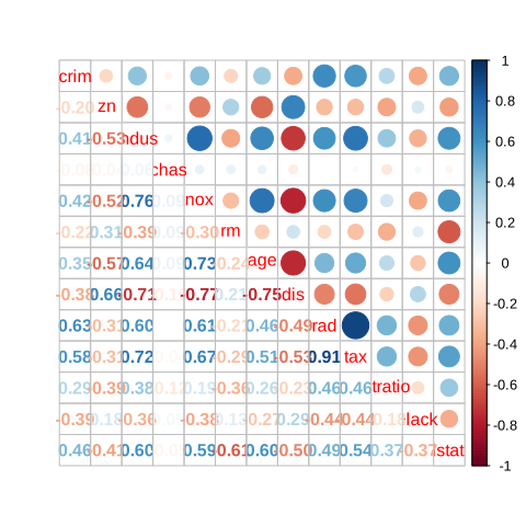

Figure 4.2: correlation matrix

we see that rad (index of accessibility to radial highways) and tax (full-value property-tax rate per $10,000) are highly correlated by \(91%\). This can be an indicator of multicollinearity.

VIF:

# we use the car package
VIFS <- car::vif(model_multi_R)

# turn the result to a data frame
vifs_df <- tibble(variables=names(VIFS))
vifs_df$vif <- VIFS[match(vifs_df$variables, names(VIFS))]
vifs_df

Table 4.4: The VIF values

variables	vif
crim	1.79
zn	2.30
indus	3.99
chas	1.07
nox	4.39
rm	1.93
age	3.10
dis	3.96
rad	7.48
tax	9.01
ptratio	1.80
black	1.35
lstat	2.94

Or we can plot the result as follows:

ggplot(vifs_df,aes(variables,vif))+
  geom_bar(stat="identity", fill="blue")+
  geom_hline(yintercept = 5, lty = 2, color="red")+
  coord_flip()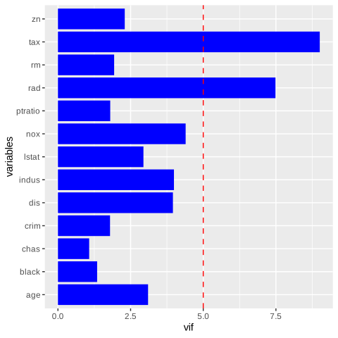

Figure 4.3: VIF values

Condition number: This index is called kappa in R.

kappa(model_multi_R)

[out] [1] 11177.64

4.3.2 Mylticollinearity remedies

As discussed before, under multicollinearity, the OLS estimates are less precise and unstable. Small changes in the data may result in significant difference in those estimates. However, since the OLS variances computed from the expression \(Var(\widehat\beta)=\sigma^2\big(X^tX\big)^{-1}\) are the minimum ones within the class of linear unbiased estimators, than the only way to shrink these variances is by manipulating the regressors matrix \(X\). To reduce multicollinearity therefore, we have two kind of methods. The first ones are the classical methods, they are just a rules of thumb to how manipulate the sample data by hands like, fore instance, removing regressors that are highly correlated to the other ones. The second ones are recent. They add some constraints on the parameters in the OLS objective function.

4.3.2.1 The classical methods

It may be easier to just return to the data at hand, and try to eliminate the multicollinearity before the final estimation (as the multicollinearity should have been detected in the first estimation ) by removing the independent variables suspected being the cause of multicollinearity, combining some variables in one variable, selecting another sample, or adding new samples if possible.

4.3.2.1.1 Variable deletion:

The easiest way to deal with multicollinearity is by removing the highly correlated regressors with some of the remaining ones from the underlying model. Therefore, if it happens that those deleted variables are irrelevant, then (as discussed in the previous chapter) the estimators of the resulted model still unbiased with the benefit of having lower standard errors than before. On the other hand, if those variables are relevant, indeed the estimators still have lower standard errors, but not unbiased, which is worse than multicollinearity. However, we can tolerate some bias if the standard errors are small enough for the estimators to be more stable.

As noted earlier, the variables of interest can be defined by the \(R^2_j\) resulted from regressing the regressor \(j\) on the remaining ones. Those regressors that have larger values than \(R^2\) of the original model will be selected to be removed. Then, we reestimate a new model with the rest of the regressors.

In R:

As a solution, we can delete the correlated variables. Since the tax and rad have larger VIF values, We can remove one of them and check again. Notice that since the VIF value of a particular regressor is based on the remaining regressors, we should remove that variable from the data, or from the model.

# remove the tax variable from the mode
model_multi_R1 <- lm(medv~. -tax, data=data_multi_R)

VIFS1 <- car::vif(model_multi_R1)

# turn the result to a data frame
vifs_df1 <- tibble(variables=names(VIFS1))
vifs_df1$vif <- VIFS1[match(vifs_df1$variables, names(VIFS1))]

Table 4.5: The VIF values

variables	vif
crim	1.79
zn	2.18
indus	3.23
chas	1.06
nox	4.37
rm	1.92
age	3.10
dis	3.95
rad	2.84
ptratio	1.79
black	1.35
lstat	2.94

Now since the model is cleaned from multicollinearity, we can reestimate the model and remove any existing insignificant variables.

result_multi_R <-  tidy(model_multi_R1, conf.int = TRUE)
result_multi_R

Table 4.6: the cleaned estimates in R

term	estimate	std.error	statistic	p.value	conf.low	conf.high
(Intercept)	34.6286431	5.1228018	6.7597078	0.0000000	24.5634261	44.6938601
crim	-0.1067339	0.0331863	-3.2162010	0.0013843	-0.1719380	-0.0415298
zn	0.0363707	0.0135129	2.6915454	0.0073539	0.0098206	0.0629208
indus	-0.0677783	0.0558291	-1.2140305	0.2253173	-0.1774706	0.0419141
chas	3.0292314	0.8636515	3.5074696	0.0004938	1.3323397	4.7261230
nox	-18.7012125	3.8466152	-4.8617321	0.0000016	-26.2589941	-11.1434309
rm	3.9116902	0.4208752	9.2941802	0.0000000	3.0847598	4.7386206
age	-0.0006054	0.0133339	-0.0454034	0.9638041	-0.0268037	0.0255929
dis	-1.4883027	0.2013809	-7.3904859	0.0000000	-1.8839734	-1.0926320
rad	0.1345757	0.0412534	3.2621690	0.0011823	0.0535214	0.2156299
ptratio	-0.9851286	0.1317385	-7.4779088	0.0000000	-1.2439668	-0.7262904
black	0.0095464	0.0027115	3.5207805	0.0004702	0.0042190	0.0148739
lstat	-0.5222095	0.0512087	-10.1976649	0.0000000	-0.6228238	-0.4215952

We are able now to remove the age and indus and display the final model.

model_multi_finalR <- lm(medv~.-tax-age-indus, data=data_multi_R)
result_multi_finalR <-  tidy(model_multi_finalR, conf.int = TRUE)
result_multi_finalR

Table 4.7: the cleaned model in R

term	estimate	std.error	statistic	p.value	conf.low	conf.high
(Intercept)	34.7123417	5.1027417	6.802684	0.0000000	24.6866381	44.7380453
crim	-0.1048430	0.0331320	-3.164402	0.0016496	-0.1699397	-0.0397463
zn	0.0366339	0.0134122	2.731393	0.0065319	0.0102821	0.0629857
chas	2.9678678	0.8608304	3.447680	0.0006136	1.2765357	4.6591999
nox	-20.3144160	3.4722917	-5.850435	0.0000000	-27.1366635	-13.4921684
rm	3.9771038	0.4077308	9.754240	0.0000000	3.1760075	4.7782002
dis	-1.4293699	0.1869222	-7.646870	0.0000000	-1.7966287	-1.0621111
rad	0.1287613	0.0407881	3.156833	0.0016922	0.0486221	0.2089005
ptratio	-1.0149139	0.1290064	-7.867159	0.0000000	-1.2683816	-0.7614463
black	0.0097001	0.0027014	3.590797	0.0003626	0.0043925	0.0150077
lstat	-0.5281470	0.0479304	-11.019036	0.0000000	-0.6223191	-0.4339748

In Python:

As we did in R, we will remove the variable TA from the model and check the VIF values. Unlike R, the function variance_inflation_factor uses the data not the model, so we should remove that variable from the data.

from statsmodels.stats.outliers_influence import variance_inflation_factor
from statsmodels.tools.tools import add_constant
import numpy as np

# create an empty data frame
vif = pd.DataFrame()

# add constant
X2 = add_constant(data_multi_py)

# delete the variable TA
del X2['TA']

# remove the dependent variable
del X2["y"]

vif['VIF'] = [variance_inflation_factor(X2.values, i) for i in range(X2.shape[1])]
vif['VIF'] = np.round(vif['VIF'], 2)
vif['variable'] = X2.columns
vif.iloc[1:,]

[out]      VIF variable
[out] 1   1.79       CR
[out] 2   2.18       ZN
[out] 3   3.23       IN
[out] 4   1.06       CH
[out] 5   4.37       NO
[out] 6   1.92       RM
[out] 7   3.10       AG
[out] 8   3.95       DI
[out] 9   2.84       RA
[out] 10  1.79       PT
[out] 11  1.35        B
[out] 12  2.94       LS

Now we can estimate the final model as we did previously.

4.3.2.1.2 Using another sample or adding new data:

Since multicollinearity is a sample feature, increase the sample size will reduce the standard errors, Ceteris Paribus, (see the formula (2.16)). However, even if new data can be available (which is not always the case), it is not guaranteed to solve the problem. This is because, in some situations, the multicollinearity resides in the functional relation of some regressors such that adding new data might make collinearity even worse.

4.3.2.1.3 Combining variables:

Sometimes, two or more variables are in a nonlinear function, so that it would be better to replace them with their cross product. For instance,, if we detect a high correlation between \(x_2\) and \(x_3\) in the model \(y_t=\beta_1+\beta_2x_{2t}+\beta_3x_{3t}+\beta_4x_{4t}+\varepsilon_t\), then the new model \(y_t=\beta_1+\beta_2(x_{2t}x_{3t})+\beta_3x_{4t}+\varepsilon_t\) could be a good alternative.

In R:

Instead of removing the variable tax (or rad), we will this time take their product.

model_comb_R <- lm(medv~crim+zn+indus+chas+nox+rm+age+dis+
                     rad:tax+ptratio+black+lstat, data=data_multi_R)
result_comb_R <-  tidy(model_comb_R, conf.int = TRUE)
result_comb_R

Table 4.8: Model with combined variables in R

term	estimate	std.error	statistic	p.value	conf.low	conf.high
(Intercept)	34.4511059	5.1777605	6.6536693	0.0000000	24.2779067	44.6243050
crim	-0.1026390	0.0333427	-3.0783079	0.0021978	-0.1681503	-0.0371277
zn	0.0351958	0.0136223	2.5836918	0.0100616	0.0084309	0.0619606
indus	-0.0735723	0.0563474	-1.3056925	0.1922661	-0.1842829	0.0371383
chas	3.0726215	0.8653211	3.5508455	0.0004208	1.3724494	4.7727936
nox	-18.2555004	3.8524776	-4.7386390	0.0000028	-25.8248003	-10.6862005
rm	3.9472716	0.4210917	9.3738993	0.0000000	3.1199158	4.7746274
age	-0.0008716	0.0133656	-0.0652131	0.9480308	-0.0271321	0.0253889
dis	-1.4812448	0.2018241	-7.3392859	0.0000000	-1.8777863	-1.0847033
ptratio	-0.9751610	0.1331557	-7.3234628	0.0000000	-1.2367837	-0.7135383
black	0.0094407	0.0027189	3.4721814	0.0005617	0.0040985	0.0147828
lstat	-0.5216097	0.0513180	-10.1642627	0.0000000	-0.6224386	-0.4207807
rad:tax	0.0001700	0.0000583	2.9181301	0.0036822	0.0000555	0.0002845

Now let us check the VIF values.

VIFS2 <- car::vif(model_comb_R)

[out] there are higher-order terms (interactions) in this model
[out] consider setting type = 'predictor'; see ?vif

# turn the result to a data frame
vifs_df2 <- tibble(variables=names(VIFS2))
vifs_df2$vif <- VIFS2[match(vifs_df2$variables, names(VIFS2))]

Table 4.9: The VIF values

variables	vif
crim	1.80
zn	2.21
indus	3.27
chas	1.06
nox	4.36
rm	1.92
age	3.10
dis	3.96
ptratio	1.82
black	1.35
lstat	2.94
rad:tax	3.06

By replacing those variables by their product, we removed collinearity.

In Python:

import statsmodels.formula.api as smf
model_multi_py = smf.ols(formula="y ~ CR+ZN+IN+CH+NO+RM+AG+DI+TA:RA+PT+B+LS", data=data_multi_py).fit()
model_multi_py.summary().tables[1]

	coef	std err	t	P>|t|	[0.025	0.975]
Intercept	34.4511	5.178	6.654	0.000	24.278	44.624
CR	-0.1026	0.033	-3.078	0.002	-0.168	-0.037
ZN	0.0352	0.014	2.584	0.010	0.008	0.062
IN	-0.0736	0.056	-1.306	0.192	-0.184	0.037
CH	3.0726	0.865	3.551	0.000	1.372	4.773
NO	-18.2555	3.852	-4.739	0.000	-25.825	-10.686
RM	3.9473	0.421	9.374	0.000	3.120	4.775
AG	-0.0009	0.013	-0.065	0.948	-0.027	0.025
DI	-1.4812	0.202	-7.339	0.000	-1.878	-1.085
TA:RA	0.0002	5.83e-05	2.918	0.004	5.55e-05	0.000
PT	-0.9752	0.133	-7.323	0.000	-1.237	-0.714
B	0.0094	0.003	3.472	0.001	0.004	0.015
LS	-0.5216	0.051	-10.164	0.000	-0.622	-0.421

4.3.2.2 The recent methods

Like the classical methods, they are also based on the idea of eliminating the effect of the suspected regressors. In other words, they allow some bias on the regression coefficients to reduce the variances. The only difference with these is that the process will be done automatically so that the bias should be at the minimum. We will briefly discuss the most popular ones, Regularization, Principal componenets, and Partial least squares.

4.3.2.2.1 Regularization (ridge and lasso):

This method merely adds some constraints on the parameters in the OLS objective function as follows (general form):

\[\begin{equation} S=\sum_i\left(y_i-x_i^t\beta\right)^2+\lambda\sum_{j=1}^k\bigg|\beta_j\bigg|^{\gamma} \tag{4.87} \end{equation}\]

Where the positive real number \(\lambda\) is considered as penalty against the parameters. In other words, it shrinks the parameters to be closer to zero. \(\gamma\) defines the form of this constraints. That is why the term Regularizaion means regularizing the OLS fit.

For simplification, we restrict our attention to the common regularization types, the ridge regression where \(\gamma=2\), and lasso regression where \(\gamma=1\).

Ridge regression RR:

When \(\gamma=2\), the formula (4.87) will be rewritten (using the symbol of the norm):

\[\begin{equation} S=\left\lVert y-X\beta\right\rVert^2+\lambda\lVert\beta\rVert^2 \tag{4.88} \end{equation}\]

It is called l2-norm regumarization (known also Tikhonov regularization)(Hilt and Seegrist 1977).

We see that the minimization must be applied to the two parts of the objective function (4.88). So if we minimize the first part alone, we will get the OLS estimates. Whereas, if we minimize the second part alone, all the estimates will be equal to zero. Together, the second part pushes the estimates to be smaller than the OLS ones, hence fewer variations. However, the effect of the constraint depends on the \(\lambda\) value. Larger values for \(\lambda\) allow the conditions to dominate the objective function, and consequently, the estimates will be closer to zero. Whereas, with smaller values of \(\lambda\), the estimates tend to the OLS ones.

Not that the expression (4.88) can be also reformulated as follows:

\[\begin{equation*} S=\left(y-X\beta\right)^t\left(y-X\beta\right)+\lambda\beta^t\beta \end{equation*}\]

Setting the differentiation equation of this function with respect to \(\beta\) to zero, we get:

\[\begin{equation*} dS=-2X^ty+2\big(X^tX\big)\beta^{*}+2\lambda\beta^{*}=0 \end{equation*}\]

Then, the ridge estimator will be:

\[\begin{equation*} \beta^*=\big(X^tX+\lambda I_k\big)^{-1}X^ty \end{equation*}\]

Since the \(\lambda\) value should be defined beforehand, this method is classified within the artificial ones. It does not care about the correlated regressors, but it shrinks the regression coefficients by the same weights. The most popular technique to define the suitable value for \(lambda\) is called cross-validation k-fold, where \(k\) is the number of the folds. With this technique, we divide the data into, say 10 folds, after has been randomly shuffled, then fit 10 different regressions such that in each regression the model uses 9 folds and keeps the last one for evaluation. In the evaluation, we usually use the mean squared errors metric MSE. The best value for \(lambda\) will be that corresponding to the minimum MSE.

It is not difficult to prove that this estimator is not unbiased.

Using \(X^ty=\big(X^tX\big)\widehat\beta\), the \(\beta^*\) can be expressed in terms of \(\widehat\beta\) as follows:

\[\begin{align*} \beta^*&=\overbrace{\big(X^tX+\lambda I_k\big)^{-1}\big(X^tX\big)}^{=\Gamma_k}\widehat\beta \\ &=\Gamma_k\widehat\beta \end{align*}\]

Its mean than will be:

\[\begin{align*} E\big(\beta^*\big)&=\Gamma_kE\big(\widehat\beta\big) \\ &=\Gamma_k\beta \\ &\not=\beta \end{align*}\]

And its variance matrix will be:

\[\begin{align*} Var\big(\beta^*\big)&=\Gamma_k \overbrace{Var\big(\widehat\beta\big)}^{=\sigma^2(X^tX)^{-1}}\Gamma_k^t \\ &=\sigma^2\big(X^tX+\lambda I_k\big)^{-1}\overbrace{\big(X^tX\big)\big(X^tX\big)^{-1}}^{I_k}\big(X^tX\big)\big(X^tX+\lambda I_k\big)^{-1} \\ &=\sigma^2\big(X^tX+\lambda I_k\big)^{-1}\big(X^tX\big)\big(X^tX+\lambda I_k\big)^{-1} \end{align*}\]

To well understand this method, let us consider the following model with mean-adjusted variables (to avoid the constant term) that are highly correlated \(y_t=\beta_1x_{1t}+\beta_2x_{2t}+\varepsilon_t\). The OLS objective function is the minimization of the sum squared of errors \(\sum\big(y_t-\beta_1x_{1t}+\beta_2x_{2t}\big)^2\). However, since the parameters have large variances, we have to set a restriction to shrink some of these parameters. Thus, the ridge regression does not allow the sum squares of the parameters to exceed a certain threshold \(c\) (that is specified by the investigator) such that \(\beta_1^2+\beta_2^2\leqslant c\). Now the minimization subjected to that constraint can be solved by using the Lagrange function as follows:

\[\begin{align*} S&=\sum\big(y_t-\beta_1x_{1t}-\beta_2x_{2t}\big)^2+\lambda\big(\beta_1^2+\beta_2^2- c\big) \\ &=\sum\big(y_t-\beta_1x_{1t}-\beta_2x_{2t}\big)^2+\lambda\big(\beta_1^2+\beta_2^2\big)-\lambda c \end{align*}\]

Since \(\lambda\) and \(c\) are both assumed to be constant, the last term \(\lambda c\) can be removed so that the objective function will be:

\[\begin{align*} S&=\sum\big(y_t-\beta_1x_{1t}-\beta_2x_{2t}\big)^2+\lambda\big(\beta_1^2+\beta_2^2\big) \end{align*}\]

Which is the same as (4.88).

In R:

To use the Ridge regression, the regressors should be first standardized such that all of them will be treated equally. Fortunately, the R package glmnet will implicitly standardize the regressors. The most important argument of the function glmnet is the weight parameter \(alpha\) that is bounded between 0 and 1. If \(alpha=1\) (which is the default), then Lasso will be used. If \(alpha=0\), Ridge will be used. Any other value in between is for elastic net. The function cv.glmnet will use cross-validation to find the best value for \(\lambda\).

suppressPackageStartupMessages(library(glmnet))

# convert data frame to matrix
X <- model.matrix(medv~. -1, data_multi_R)

# create cross validation in glmnet
set.seed(111)
cv_mod <- cv.glmnet(X, data_multi_R$medv, family="gaussian", alpha=0)

Now we can extract the best value of lambda as follows:

cv_mod$lambda.min

[out] [1] 0.6777654

We then use that value in the model.

# we use that value
model_ridge_R <- glmnet(X, data_multi_R$medv, family="gaussian", alpha=0, lambda=cv_mod$lambda.min)
coef(model_ridge_R)

[out] 14 x 1 sparse Matrix of class "dgCMatrix"
[out]                        s0
[out] (Intercept)  28.051686825
[out] crim         -0.087904300
[out] zn            0.032606201
[out] indus        -0.038328191
[out] chas          2.902980774
[out] nox         -12.005369287
[out] rm            4.014163735
[out] age          -0.003862644
[out] dis          -1.120903830
[out] rad           0.154161048
[out] tax          -0.005729860
[out] ptratio      -0.855862908
[out] black         0.009068108
[out] lstat        -0.471596371

In Python:

To fit a regularized model, we will stick with the statsmodels. However, to choose the best value for \(\lambda\), we will implement cross validation in the scikit learn package which is designed for machine learning models.

from sklearn.linear_model import RidgeCV
from sklearn.preprocessing import StandardScaler

X_py = data_multi_py[list(data_multi_py.columns[:-1])]
y_py = data_multi_py["y"]
# NOTE: scikit-learn removed the normalize= argument in v1.2, and no longer
# accepts alpha = 0. We standardize the regressors explicitly instead, and the
# grid keeps 1e-5 which is effectively unregularized.
grid = [1e-5, 1e-4, 1e-3, 1e-2, 1e-1, 1.0, 10.0, 100.0]
X_py_scaled = StandardScaler().fit_transform(X_py)
ridge_cv = RidgeCV(alphas=grid, cv=5).fit(X_py_scaled, y_py)

We get access to the best value as follows:

ridge_cv.alpha_

[out] 100.0

Then, we will use that value in our final model. But first, we should standardize the variables.

from sklearn.preprocessing import StandardScaler
sc = StandardScaler()
scaled = sc.fit_transform(data_multi_py)

X_py = scaled[:, :-1]
y_py = scaled[:, -1]

We will use the statsmodels package to fit the model.

import statsmodels.api as sm

# plug in the value 0.1 and fit the modle
model_ridge_py = sm.OLS(y_py, X_py, data=scaled).fit_regularized(alpha=0.1,  L1_wt=0)
ridge_result = pd.DataFrame({"variables":list(data_multi_py.columns[:-1]), "ridge_coeff":model_ridge_py.params})
ridge_result

[out]    variables  ridge_coeff
[out] 0         CR    -0.078558
[out] 1         ZN     0.076445
[out] 2         IN    -0.033648
[out] 3         CH     0.080625
[out] 4         NO    -0.135443
[out] 5         RM     0.307361
[out] 6         AG    -0.013958
[out] 7         DI    -0.236235
[out] 8         RA     0.123494
[out] 9         TA    -0.090851
[out] 10        PT    -0.195973
[out] 11         B     0.089016
[out] 12        LS    -0.355435

Least absolute shrinkage and selection operator LASSO:

In this type of regularization, which is also called l1-norm, we set \(\gamma=1\). The objective function will be:

\[\begin{equation} S=\left\lVert y-X\beta\right\rVert^2+\lambda\lVert\beta\rVert_1 \tag{4.89} \end{equation}\] Where \(\lVert\beta\rVert_1=\sum_{j=1}^{k}\big|\beta_j\big|\).

This method shrinks the sum of the absolute values of the parameters to zero. However, unlike the ridge method that shrinks the estimates to be closer to zero but not equal to zero, LASSO sets some of which exactly to zero, then leaves the remaining ones with their large values. In other words, variables associated with zero coefficients will be removed from the model. That is why this method is attractive to use in applications where the number of features (regressors) is much larger than the sample size (in medicine, for instance ). Moreover, the number of features with no zero coefficients is at most equal to \(Min(n,k)\), hence obtaining one possible solution, unlike the OLS that will give multiple ones in that situation.

Using the above example, the LASSO objective function will be:

\[\begin{align*} S&=\sum\big(y_t-\beta_1x_{1t}-\beta_2x_{2t}\big)^2+\lambda\big(\big|\beta_1\big|+\big|\beta_2\big|\big) \end{align*}\]

The minimization of this expression results in either:

• \(\widehat\beta_1=0\) and \(\big|\widehat\beta_2\big|\geqslant0\).
• \(\widehat\beta_2=0\) and \(\big|\widehat\beta_1\big|\geqslant0\).

There exist several techniques that have sprung up from LASSO:

• Fussed Lasso((Robert.T et al. 2005)): Penalizes both the coefficients and their differences by the following expression:

\[\begin{equation*} S=\big(y-X\beta\big)^t\big(y-X\beta\big)+\lambda_1\sum_{j=1}^k\big|\beta_j\big|+\lambda_2\sum_{j=1}^k\big|\beta_j-\beta_{j-1}\big| \end{equation*}\]

• Elastic net: uses a mix between LASSO and RR as follows:

\[\begin{equation*} S=\big(y-X\beta\big)^t\big(y-X\beta\big)+\lambda_1\sum_{j=1}^k\big|\beta_j\big|+\lambda_2\sum_{j=1}^k\beta_j^2 \end{equation*}\]

• Adaptive Lasso: encourages more shrinkage for larger coefficients by adding small weights as follows:

\[\begin{equation*} S=\big(y-X\beta\big)^t\big(y-X\beta\big)+\lambda_1\sum_{j=1}^k\big|\beta_j\big|+\lambda_2\sum_{j=1}^kw_j\big|\beta_j\big| \end{equation*}\]

where \(w_j=\frac{1}{\big|\beta_j\big|}\)

In R:

For lasso regression, the value of alpha should be equal to one , which is the default.

# create cross validation in glmnet
set.seed(222)
cv_mod2 <- cv.glmnet(X, data_multi_R$medv, family="gaussian", alpha=1)
cv_mod2$lambda.min

[out] [1] 0.02800535

Then we use that value in our model.

# we use that value

model_lasso_R<- glmnet(X, data_multi_R$medv, family="gaussian", alpha=1, lambda=cv_mod2$lambda.min)
coef(model_lasso_R)

[out] 14 x 1 sparse Matrix of class "dgCMatrix"
[out]                        s0
[out] (Intercept)  34.548175599
[out] crim         -0.098693203
[out] zn            0.041588291
[out] indus         .          
[out] chas          2.681633344
[out] nox         -16.354590598
[out] rm            3.860035926
[out] age           .          
[out] dis          -1.399697121
[out] rad           0.255484621
[out] tax          -0.009935509
[out] ptratio      -0.931031828
[out] black         0.009031422
[out] lstat        -0.522741592

As we see, the less relevant variables have been removed, indus, age. That is why this method is also called feature selection method.

Now let us compare the estimates of the last two models with those of the original one. But we should first refit the original model with scaled variables.

# standardize the data
scaled_multi_R <- data.frame(scale(data_multi_R))

# we do not need the intercept with scaled variables
model_multi_R_sc <- lm(medv~. -1, data=scaled_multi_R)
result_multi <-  tidy(model_multi_R, conf.int = TRUE)
df_origin <- result_multi[, c("term", "estimate")]
names(df_origin) <- c("variables", "coef_origin")

df_ridge <-data.frame(matrix(coef(model_ridge_R)))
names(df_ridge)[1] <- "coef_ridge"

# add intercept to column names
df_ridge["variables"] <- c("(Intercept)", names(data_multi_R)[-length(names(data_multi_R))])

# reorder columns
df_ridge <- df_ridge[,c(2,1)] 

df_lasso <-data.frame(matrix(coef(model_lasso_R)))
names(df_lasso)[1] <- "coef_lasso"

# add intercept to column names
df_lasso["variables"] <- c("(Intercept)", names(data_multi_R)[-length(names(data_multi_R))])

# reorder columns
df_lasso <- df_lasso[,c(2,1)] 

# put everything in one data frame
one_df_R <- merge(merge(df_origin, df_ridge, by="variables"), df_lasso, by="variables")

# do not need the intercept
one_df_R[-c(1),]

[out]    variables   coef_origin    coef_ridge    coef_lasso
[out] 2        age  6.922246e-04  -0.003862644   0.000000000
[out] 3      black  9.311683e-03   0.009068108   0.009031422
[out] 4       chas  2.686734e+00   2.902980774   2.681633344
[out] 5       crim -1.080114e-01  -0.087904300  -0.098693203
[out] 6        dis -1.475567e+00  -1.120903830  -1.399697121
[out] 7      indus  2.055863e-02  -0.038328191   0.000000000
[out] 8      lstat -5.247584e-01  -0.471596371  -0.522741592
[out] 9        nox -1.776661e+01 -12.005369287 -16.354590598
[out] 10   ptratio -9.527472e-01  -0.855862908  -0.931031828
[out] 11       rad  3.060495e-01   0.154161048   0.255484621
[out] 12        rm  3.809865e+00   4.014163735   3.860035926
[out] 13       tax -1.233459e-02  -0.005729860  -0.009935509
[out] 14        zn  4.642046e-02   0.032606201   0.041588291

As we see, some coefficients have been shrunk, while some others have not. This is expected since this method shrinks the sum square of coefficients as a whole, not each individual one. Notice that the two variables tax and rad that cause multicollinearity have been heavily shrunk.

In Python:

from sklearn.linear_model import LassoCV

lasso_cv = LassoCV(cv=5, random_state=0).fit(X_py, y_py)
m=lasso_cv.alpha_
m

[out] 0.017040965723789027

Plug in then that value and fit the model

model_lasso_py = sm.OLS(y_py, X_py, data=scaled).fit_regularized(alpha=m,  L1_wt=1)

# put the results in a data frame
lasso_result = pd.DataFrame({"variables":list(data_multi_py.columns[:-1]), "lasso_coeff":model_lasso_py.params})
lasso_result

[out]    variables  lasso_coeff
[out] 0         CR    -0.041106
[out] 1         ZN     0.055578
[out] 2         IN     0.000000
[out] 3         CH     0.070670
[out] 4         NO    -0.136573
[out] 5         RM     0.321589
[out] 6         AG     0.000000
[out] 7         DI    -0.218068
[out] 8         RA     0.000000
[out] 9         TA     0.000000
[out] 10        PT    -0.194112
[out] 11         B     0.075048
[out] 12        LS    -0.405335

As we see, the less relevant variables have been removed, In, AG, and the variables TA, RA that causes multicollinearity.

We can compare the original model to these two last ones. But first we should get the original coefficients with scaled regressors instead.

import statsmodels.api as sm
from sklearn.preprocessing import StandardScaler
sc=StandardScaler()
data_scaled = sc.fit_transform(data_multi_py)
X1 = data_scaled[:, :-1]
y1 = data_scaled[:, -1]
model_multi_py_sc = sm.OLS(y1, X1, data=data_scaled).fit()
multi_result = pd.DataFrame({"variables":data_multi_py.columns[:-1], "coefficients":model_multi_py_sc.params})

# put every thing in one data frame
one_df =pd.concat([multi_result, ridge_result.ridge_coeff, lasso_result.lasso_coeff], axis=1) 
one_df

[out]    variables  coefficients  ridge_coeff  lasso_coeff
[out] 0         CR     -0.101017    -0.078558    -0.041106
[out] 1         ZN      0.117715     0.076445     0.055578
[out] 2         IN      0.015335    -0.033648     0.000000
[out] 3         CH      0.074199     0.080625     0.070670
[out] 4         NO     -0.223848    -0.135443    -0.136573
[out] 5         RM      0.291056     0.307361     0.321589
[out] 6         AG      0.002119    -0.013958     0.000000
[out] 7         DI     -0.337836    -0.236235    -0.218068
[out] 8         RA      0.289749     0.123494     0.000000
[out] 9         TA     -0.226032    -0.090851     0.000000
[out] 10        PT     -0.224271    -0.195973    -0.194112
[out] 11         B      0.092432     0.089016     0.075048
[out] 12        LS     -0.407447    -0.355435    -0.405335

4.3.2.2.2 Principal components PC

Since the multicollinearity resides in the matrix \(X^tX\), we can think to extract orthogonal features from the original ones using what is called diagonalization as follows:

\[\begin{equation*} X^tX=V\Lambda V^t \end{equation*}\]

Where \(\Lambda\) is a diagonal matrix that contains the eigenvalues of \(X^tX\) , and \(V\) is an orthogonal matrix that has the eigenvectors associated with the \(X^tX\). That is \(VV^t=V^tV=I\).

Let us consider our standard model:

\[\begin{equation*} y=X\beta+\varepsilon \end{equation*}\]

Using the property \(VV^t=I\)

\[\begin{align} y&=XVV^t\beta+\varepsilon \notag \\ &=\overbrace{\big(XV\big)}^{W}\overbrace{\big(V^t\beta\big)}^{\alpha}+\varepsilon \notag \\ &=W\alpha+\varepsilon \\ \tag{4.90} \end{align}\]

Where the matrix \(W\) has the orthogonally transformed variables called The principal components (or Factors), and \(\alpha\) has corresponding estimates.

The OLS estimator then will be:

\[\begin{align} \widehat\alpha&=\big(W^tW\big)^{-1}W^ty \notag \\ &=\big(V^tX^tXV\big)^{-1}V^tX^ty \notag \\ &=\big(\overbrace{V^tV}^{I_k}\Lambda \overbrace{V^tV}^{I_k}\big)^{-1}V^tX^ty \notag \\ &=\Lambda^{-1}V^tX^ty \tag{4.91} \end{align}\]

And its variance matrix will be:

\[\begin{align} Var(\widehat\alpha)&=\sigma^2\big(W^tW\big)^{-1} \notag \\ &=\sigma^2\Lambda^{-1} \tag{4.92} \end{align}\]

Since the variance matrix is diagonal (the covariances are all equal to zero), the resulted coefficients should have the desired properties (the minimum standard errors). The main attractive property of this technique is that a small subset of the first components (corresponding to the few first larger eigenvalues) can capture the most information contained in the original regressors. That is why this technique is classified within the dimension reduction methods, notably used when the number of regressors is greater than the sample size, in which the OLS method fails.

We can briefly explain how PC works as follows:

With \(n\) observations and \(k\) regressors, we will get scatter points in a k-dimensional space. The PC starts by orthogonally projecting the points onto a line (that must pass by the origin) that minimizes the distances (see the graph below) in the sense of the least-squares, or equivalently maximizes the distance between the projected point and the origin. This line is the first principal component. To find the next principal component, the PC finds, in the same way, the next line, except that this line now must be orthogonal to the previous one. By doing so, the second principal component will maximize the rest of the variation that is not captured by the previous component. Continuing doing so until the rest of the variations is small enough to be neglected.

[out] Warning in fortify(data, ...): Arguments in `...` must be used.
[out] ✖ Problematic argument:
[out] • na.rm = TRUE
[out] ℹ Did you misspell an argument name?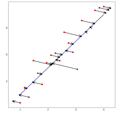

Figure 4.4: Orthogonal projection of PC

It should be noted that the matrix \(X\) should be first standardized before applying the PC method to ensure that all the regressors will be treated equally, and no variable can dominate the others because of its large magnitude.

However, even multicollinearity is now entirely removed from the new model with the principal components as regressors, and the new regression coefficients are precisely estimated with higher accuracy, another more serious problem arises here about the interpretation of those coefficients. Since the linear combination of the original regressors for each component is computed by maximizing the variations among the regressors, there is nothing taken into account about the relations between the original regressors and the dependent variable. In other words, The PC method is optimum to explain the matrix \(X\) rather than the dependent variable \(y\) (or the matrix of the dependent variables \(Y\) like in SEM models), in which we will not be sure that these new regressors are relevant for \(y\) or not.

for more detail about this method see(Marc.P et al. 2020).

In R:

The R package pls is designed to fit a model with principal components. In the function pcr , we should set the argument scale to TRUE to standardize the variables before constructing the principal components. This function uses also cross-validation to define the best model (based on the RMSE metric)

suppressPackageStartupMessages(library(pls))
set.seed(111)
model_pcr_R <- pcr(medv ~ ., data=data_multi_R, scale=TRUE, validation="CV")
summary(model_pcr_R)

[out] Data:     X dimension: 506 13 
[out]   Y dimension: 506 1
[out] Fit method: svdpc
[out] Number of components considered: 13
[out] 
[out] VALIDATION: RMSEP
[out] Cross-validated using 10 random segments.
[out]        (Intercept)  1 comps  2 comps  3 comps  4 comps  5 comps  6 comps
[out] CV           9.206    7.293    6.842    5.575    5.518    5.114    5.092
[out] adjCV        9.206    7.291    6.843    5.566    5.585    5.107    5.087
[out]        7 comps  8 comps  9 comps  10 comps  11 comps  12 comps  13 comps
[out] CV       5.109    5.101    5.124     5.156     5.171     4.965     4.890
[out] adjCV    5.105    5.095    5.118     5.152     5.160     4.954     4.878
[out] 
[out] TRAINING: % variance explained
[out]       1 comps  2 comps  3 comps  4 comps  5 comps  6 comps  7 comps  8 comps
[out] X       47.13    58.15    67.71    74.31    80.73    85.79    89.91    92.95
[out] medv    37.42    45.59    63.59    64.78    69.70    70.05    70.05    70.56
[out]       9 comps  10 comps  11 comps  12 comps  13 comps
[out] X       95.08     96.78     98.21     99.51    100.00
[out] medv    70.57     70.89     71.30     73.21     74.06

This output has two tables. The first table shows the RMSE values computed with cross-validation each time we add a component. Starting the model has only the intercept, and ending with the total number that is equal to the number of the regressors we have in the data. The second table shows the variance of our dependent variable (in percentage) explained by the components add in the model. For instance, the first component explains \(47.13%\), the second \(58.15\), and so on. We see that we do not gain much after the \(8^{th}\) one.

We can plot the validation process as follows.

validationplot(model_pcr_R)

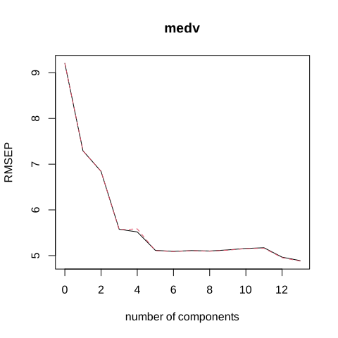
Figure 4.5: RMSE values for each PC added

Now if we want to use this model for prediction, we just need to specify the desired number of components. Say, for instance, we want to get the fitted values using only the first 4 components.

pre_medv <- predict(model_pcr_R, data_multi_R[, -c(length(data_multi_R))], ncomp=4)

# call the rmse metric from the package metrics (should be installed)
Metrics::rmse(data_multi_R$medv,pre_medv)

[out] [1] 5.453034

Which is closer to that computed from cross-validation.

In Python:

For Python we will use sklearn package. We standardize the features with the function StandarScaler. Then we use the function PCR to extract components. Finally, we use LinearRegression to fit the model.

from sklearn.preprocessing import StandardScaler
from sklearn.decomposition import PCA
from sklearn.linear_model import LinearRegression
from sklearn.metrics import mean_squared_error

# scale the variables
sc=StandardScaler()
data_scaled = sc.fit_transform(data_multi_py)
X1 = data_scaled[:, :-1]
y1 = data_scaled[:, -1]

Since the sklearn models mostly used for prediction purposes, we will held out some sample to figure out what is the best number of PC that should be included.

from sklearn.model_selection import train_test_split
import numpy as np

x_train, x_test, y_train, y_test= train_test_split(X1, y1, test_size = 0.2, random_state=111)

# extract PC
pca = PCA().fit(x_train)
X_pca_train = pca.transform(x_train)
x_pca_test = pca.transform(x_test)

# fit a linear model each time we add a component.
MSE = []
for i, _ in enumerate(data_multi_py.columns[:-1], start=1):
  lr = LinearRegression()
  model = lr.fit(X_pca_train[:, :i], y_train)
  # use the test data to compute MSE
  y_pred = model.predict(x_pca_test[:, :i])
  MSE.append(mean_squared_error(y_test, y_pred))

# extract the minimum value 
np.round(MSE, 4)

[out] array([0.7014, 0.5537, 0.4015, 0.3407, 0.3254, 0.3266, 0.3291, 0.3384,
[out]        0.347 , 0.345 , 0.3418, 0.2904, 0.2732])

Starting from the \(5^{th}\) (0.3254), we do not gain much (except for the two last ones).

Now we can fit a final model with the first 5 components, and display the regression coefficients.

pca = PCA().fit(X1)
X_pca = pca.transform(X1)

lr = LinearRegression()
model_pcr_py = lr.fit(X_pca[:, :5], y1)

# display the coefficients
model_pcr_py.coef_

[out] array([-0.24714505,  0.23865268,  0.38066188, -0.11750262, -0.24280294])

4.3.2.2.3 Partial least squares PLS

To overcome the limitations of the above technique, PLS provides much information about the relations between the regressors and the dependent variables as well as the relations among regressors. It is commonly used for models that have many dependent variables, such as SEM. The idea behind this technique is the same as PC with the difference that now we search for components, called latent vectors, by maximizing the covariance between \(X\) and \(Y\), then using them in a linear model to predict \(Y\). Briefly, this technique extracts factors for both \(X\) and \(Y\) so that the covariance between those factors is maximized, then regressing the \(Y\) factors on the \(X\) factors. Formally speaking, in this technique instead of extracting the eigenvectors of \(X\) from the matrix \(X^tX\) as we do in the PC, the eigenvectors of \(X\) will be extracted from the matrix \(X^tYY^tX\), and those of \(Y\) will be extracted from the matrix \(Y^tXX^tY\).
Let \(X\) be \((n\times k)\) matrix, and \(Y\) be \((n\times q)\) matrix. Each matrix then will be expressed as follows:

\[\begin{equation} \begin{cases} X=TP^t+\varepsilon_x\\ Y=\Pi Q^t+\varepsilon_y \tag{4.93} \end{cases} \end{equation}\]

Where \(\underset{(n\times r)}{T}\) is called \(X\)-scores, \(\underset{(n\times r)}{\Pi}\) is called \(Y\)-scores, \(\underset{(k\times r)}{T}\) is called \(X\)-loadings, \(\underset{(q\times r)}{Q}\) is called \(Y\)-loadings, and \(\varepsilon_x\), \(\varepsilon_y\) are residuals.

An iterative process then will extract the \(X\)-scores \(t\) and \(Y\)-scores \(\pi\) at each iteration so that \(cov(t,\pi)\) should be maximum.

To apply this method, there exist many algorithms. The classical one is called the nonlinear iterative squares NIPALS. It looks for a weight vector (eigenvectors) that will be used to deflate the values of \(X\) and \(Y\) in each step. Those steps can be summarized as follows:

• Initialization of \(Y\)-score and \(\pi\) by any random values.
• Computing the weight vector \(w\) using \(w=\frac{X^t\pi}{\pi^t\pi}\).
• Computing the factor value \(t\) using \(t=Xw\).
• Computing the weight vector \(c\) using \(w=\frac{Y^tt}{t^tt}\).
• Computing the new value of \(\pi\) using \(\pi=Yc\)

Iterating over these steps until convergence of \(\pi\).

In the case of one single dependent variable, the matrix \(Y\) reduces to the vector \(y\), the above values then converge in one single iteration. PLS with one dependent variable is known as PLS1. Otherwise, it is called PLS2.

At the end of each iteration, the values of \(X\) and \(Y\) from the previous iteration will be deflated by (note that the way of deflating gives many variants of PLS, hence many algorithms):

\[\begin{equation} \begin{cases} X_i=X_{i-1}-t_iw^t\\ Y_i=X_{i-1}-\pi_ic^t \tag{4.94} \end{cases} \end{equation}\]

And so on with the next iteration until the matrix, \(X\) reduces to the null matrix.

Once all the factors of both matrices are extracted, we can now perform a regression model for \(Y\) by first fit the following model:

\[\begin{equation} \Pi=T\beta^*+H \tag{4.95} \end{equation}\]

Where \(H\) is made up of residuals.

Then substituting the estimated model into (4.93) as follows (note that at the end of the algorithm, the matrix \(X\) reduces to the null matrix which makes \(\varepsilon_x=0\)):

\[\begin{align} Y&=\Pi Q^t+\varepsilon_y \notag \\ &=\big(T\beta^*+H\big)Q^t+\varepsilon_y \notag \\ &= T\beta^* Q^t+HQ^t+\varepsilon_y \notag \\ &=XP\beta^* Q^t+\varepsilon \tag{4.96} \end{align}\]

Since \(\beta^*\), \(P\), and \(Q\) are all known, we can readily predict \(Y\).

The algorithm NIPALS can be also used in PC technique to extract the factors by applying the following steps in each iteration (starting by initializing \(t\) by any random value):

• Computing \(w=\frac{1}{\lambda_w}X^tt\). (using \(X^tXw=\lambda_ww\))
• Computing \(t=Xw\).

Stop when \(t\) converges.

For more depth on this method see(Saikat.M and Jun.Y 2008).

In R:

As we did in PCR, we will again use the R package pls. But this time we will call the function plsr instead, with almost the same arguments (for standardization and cross-validation).

set.seed(222)
model_pls_R <- plsr(medv ~ ., data=data_multi_R, scale=TRUE, validation="CV")
summary(model_pls_R)

[out] Data:     X dimension: 506 13 
[out]   Y dimension: 506 1
[out] Fit method: kernelpls
[out] Number of components considered: 13
[out] 
[out] VALIDATION: RMSEP
[out] Cross-validated using 10 random segments.
[out]        (Intercept)  1 comps  2 comps  3 comps  4 comps  5 comps  6 comps
[out] CV           9.206    6.543    5.068    4.970    4.921    4.880    4.845
[out] adjCV        9.206    6.541    5.063    4.963    4.911    4.869    4.837
[out]        7 comps  8 comps  9 comps  10 comps  11 comps  12 comps  13 comps
[out] CV       4.836    4.838    4.831     4.832     4.833     4.833     4.833
[out] adjCV    4.828    4.829    4.823     4.824     4.825     4.825     4.825
[out] 
[out] TRAINING: % variance explained
[out]       1 comps  2 comps  3 comps  4 comps  5 comps  6 comps  7 comps  8 comps
[out] X       45.86    56.78    63.91    69.70    75.47    78.72    81.95    84.62
[out] medv    49.93    70.64    72.30    73.29    73.77    73.92    74.01    74.06
[out]       9 comps  10 comps  11 comps  12 comps  13 comps
[out] X       90.16     92.40     96.22     98.16    100.00
[out] medv    74.06     74.06     74.06     74.06     74.06

Using the same reasoning as in PCR, the \(RMSE\) does not drop much from the \(7^{th}\) component. While for the explained variance does not go up much after the \(9^{th}\) component.

In Python:

sklearn package has the function PLSRegression to fit PLS models.

from sklearn.cross_decomposition import PLSRegression

MSE=[]
for i, _ in enumerate(data_multi_py.columns[:-1], start=1):
    pls = PLSRegression(n_components=i)
    model = pls.fit(x_train, y_train)
    y_pred = model.predict(x_test)
    MSE.append(mean_squared_error(y_test, y_pred))

# extract the minimum value 
np.round(MSE, 4)

[out] array([0.5741, 0.3137, 0.3111, 0.296 , 0.2919, 0.2739, 0.2734, 0.2722,
[out]        0.2725, 0.2731, 0.2733, 0.2732, 0.2732])

The results are slightly different from R. Here the best number of components is \(8\) (\(0.2722\)). We can then fit the final model with the whole data.

pls = PLSRegression(n_components=8)
model_pls_py =pls.fit(X1,y1)
model_pls_py.coef_

[out] array([[-0.10256622,  0.11500432,  0.01764839,  0.07147925, -0.23076471,
[out]          0.29436832,  0.00173599, -0.3382073 ,  0.28644755, -0.21862333,
[out]         -0.23084729,  0.09296234, -0.40207619]])