6.2 Quantile regression
In some applications, the dependent variable is not linear in the parameters, but the quantile of that variable is linear so that the original model would be:
\[\begin{equation} Q_q(y)=X\beta+\varepsilon \tag{6.25} \end{equation}\]
For a specific quantile \(q\).
Or equivalently in terms of probability:
\[\begin{equation} P\bigg(y\leqslant X\beta \big|X\bigg)=q \tag{6.26} \end{equation}\]
That means that taking a randomly an observation from the population, the probability of \(y_i \leqslant x_i^t\beta\) (which is the error \(\varepsilon_i\)) will be equal to \(q\), otherwise will be equal to \(1-q\).
Using Bernoulli distribution, the function to minimize is the following:
\[\begin{equation} S_q\big(\beta)=\sum\limits_{y_i\geqslant x_i^t\beta} q\big|y_i-x_i^t\beta\big|+\sum\limits_{y_i\leqslant x_i^t\beta} (1-q)\big|y_i-x_i^t\beta\big| \tag{6.27} \end{equation}\]
Such as NLS objective function, solving this one requires also numerical methods.
Definition 6.3 (Quantiles) The \(q^{th}\) quantile of a random variable with distribution function \(F\) is deined by:
\[\begin{equation*} Q_q=inf\{{x: F(x)\geqslant q}\} \quad\text{for} \quad q \in[0,1] \end{equation*}\]
The quantile estimator \(\beta_Q\) is consistent and asymptotically normally distributed with the following covariance matrix(Buchinsky 1998):
\[\begin{equation} Var_{asy}\big(\beta_Q\big)=\frac{1}{n}H^{-1}GH^{-1} \tag{6.28} \end{equation}\]
Where
\[\begin{equation*} H=plim\frac{1}{n}\sum\limits_{i=1}^nf_Q\big(0\big|x_i)x_ix_i^t \end{equation*}\]
And
\[\begin{equation*} G=plim\frac{q(1-q)}{n}\sum\limits_{i=1}^nx_ix_i^t \end{equation*}\]
6.2.0.1 Least absolute deviation LAD
Least absolute deviation is a special case of quantile regression when \(q=0.5\), which is called also Median rgression, L1-norm. Since the median is a robust measure that is not affected by outliers, this type of regression is well suited for data with outliers. the objective function then can be derived from (6.27) as follows:
\[\begin{equation} S_{LAD}\big(\beta)=\sum\limits_{i=1} \big|y_i-x_i^t\beta\big| \tag{6.29} \end{equation}\]
That regression can be seen as the OLS regression with the assumption that the distribution function of the disturbances has its median equal to zero (instead of the mean in the OLS regression), \(med(\varepsilon)=0\) ( assuming fixed regressors, otherwise, the conditional median equal to zero \(med(\varepsilon|X)=0\)). As such, the original model would be:
\[\begin{equation} med(y|X)=X\beta \tag{6.30} \end{equation}\]
Using the expression (6.28) with the orthogonality assumption such that \(f\big(0\big|x_i)=f\big(0\big)\), the asymptotic variance will be given by:
\[\begin{align} Var_{Asy}\big(\beta_{LAD}\big)&=\frac{1}{n}\bigg[plim\frac{1}{n}\sum\limits_{i=1}^nf\big(0\big)x_ix_i^t\bigg]^{-1}\bigg[plim \frac{0.25}{n}\sum\limits_{i=1}^nx_ix_i^t\bigg]\bigg[plim\frac{1}{n}\sum\limits_{i=1}^nf\big(0\big)x_ix_i^t\bigg]^{-1} \notag \\ &=\frac{0.25\bigg[plim \frac{1}{n}\sum\limits_{i=1}^nx_ix_i^t\bigg]^{-1}}{f\big(0\big)^2} \tag{6.31} \end{align}\]
The LAD estimator is asymptotically normally distributed (Hansen 2018):
\[\begin{equation} \sqrt n \big(\beta_{LAD}-\beta\big)\overset{d}{\rightarrow}\mathrm N\big(0, V) \tag{6.32} \end{equation}\]
Where \(V\) is the above variance (6.31).
As we see, the variance depends on the density function of errors \(f(.)\) that is in most cases unknown. However, this density can be estimated using the nonparametric kernel density estimation (Green 2018) as follows:
\[\begin{equation} \widehat f(0)=\frac{1}{n}\sum\limits_{i=1}^n\frac{1}{h}K\Bigg(\frac{e_i}{h}\Bigg) \tag{6.33} \end{equation}\]
Where \(h\) is the bandwidth, \(K()\) is a kernel function (the logit kernel is the common choice).
For hypothesis testing, we can use the same approach used in the OLS method. OLS method uses the difference between the constrained sum squared errors and the unconstrained counterpart one. we showed in 3.9.2 that that difference follows the \(\chi^2_{q}\), where the null hypothesis was \(\underset{(q\times k)}{R}\underset{(k\times 1)}{\beta}=\underset{(q\times 1)}{r}\). That difference in LAD regression should be:
\[\begin{equation} S_{LAD}=\underset{\beta_R}{Min}\sum\limits^{n}_{i=1}\big|y_i-x^t_i\beta\big|-\underset{\beta}{Min}\sum\limits^{n}_{i=1}\big|y_i-x^t_i\beta\big| \tag{6.34} \end{equation}\]
As discussed above, the approximate distribution of the statistic \(S_{LAD}\) is \(\frac{0.25\chi^2_{k-q}}{\widehat f(0)}\).
However, there exists another alternative for obtaining an approximation distribution without the need to estimate the density function is that provided by (Chen et al. 2008).
The authors suggest first solving the minimum of each member of the right hand side of (6.34) separately, using the classical linear programming. So that the first member becomes:
\[\begin{equation} \begin{cases} Min\sum\limits_{i=1}^na_i \\ S.C \\ R\beta=r \\ a_i\leqslant y_i-x^t_i\beta \\ a_i\geqslant y_i-x^t_i\beta \end{cases} \tag{6.35} \end{equation}\]
That gives \(\beta_R^{LAD}\), and the second member:
\[\begin{equation} \begin{cases} Min\sum\limits_{i=1}^na_i \\ S.C \\ a_i\leqslant y_i-x^t_i\beta \\ a_i\geqslant y_i-x^t_i\beta \end{cases} \tag{6.36} \end{equation}\]
That gives \(\beta^{LAD}\).
Next, They provided the following statistic instead
\[\begin{equation} \begin{split} S^*_{LAD}&=\underset{\beta_R}{Min}\sum\limits^{n}_{i=1}w_i\big|y_i-x^t_i\beta\big|-\underset{\beta}{Min}\sum\limits^{n}_{i=1}w_i\big|y_i-x^t_i\beta\big| \\ &-\bigg(\sum\limits^{n}_{i=1}w_i\big|y_i-x^t_i\beta_R^{LAD}\big|-\sum\limits^{n}_{i=1}w_i\big|y_i-x^t_i\beta^{LAD}\big|\bigg) \end{split} \tag{6.37} \end{equation}\]
Where \(w_i\) is a random variable independently and identically distributed with mean and variance both equal to one.
By repeatedly generating a large number of sequences \(w_i\), the empirical distribution of \(S^*_{LAD}\) converges to that of \(S_{LAD}\) without having to estimate \(f(0)\).
In R:
For quantile regression, we will use the R package quantreg. The data we will be using is called engel, provided by this package. This data has 235 observations with two variables, income and expenditure on food for Belgian working class households.
library(quantreg)
data(engel)
engel <-tibble(engel)
kbl(head(engel), booktabs = T, align = "c", col.names = gsub("[.]", " ", names(engel))) %>%
  kable_styling(latex_options = c("striped", "hold_position"),
full_width = F)| income | foodexp |
|---|---|
| 420.1577 | 255.8394 |
| 541.4117 | 310.9587 |
| 901.1575 | 485.6800 |
| 639.0802 | 402.9974 |
| 750.8756 | 495.5608 |
| 945.7989 | 633.7978 |
The tau argument in rq function is where we specified the quantile. Let us, for instance, use the \(25%\) quantile:
mod_reg_r <- rq(engel$foodexp~engel$income, tau=0.25)
kbl(broom::tidy(mod_reg_r), booktabs = T, align = "c") %>%
  kable_styling(latex_options = c("striped", "hold_position"),
full_width = F)| term | estimate | conf.low | conf.high | tau |
|---|---|---|---|---|
| (Intercept) | 95.4835396 | 67.5662860 | 134.9199638 | 0.25 |
| engel$income | 0.4741032 | 0.4168149 | 0.5112239 | 0.25 |
As we see, the estimates are both significant since the confidence interval does not contain zero.
This function uses by default the br algorithm (among others) which stands for Barrodale and Roberts algorithm.
To perform a LAD regression we should set the \(tau=0.5\).
The following plot shows the difference between OLS regression and the LAD regression:
mod_reg2_r <- rq(engel$foodexp~engel$income, tau=.5)
outliers <-dplyr::filter(engel, income > 2500 & foodexp < 2000 )

ggplot(data=engel, aes(income, foodexp))+
  geom_point()+
  geom_point(data=outliers, aes(x=income, y= foodexp), color="red", size=3)+
  xlab("Income")+
  ylab("Food Expenditure")+
  geom_smooth(method="lm", color="red", se=FALSE)+
  geom_abline(intercept = mod_reg2_r$coefficients[1], slope = mod_reg2_r$coefficients[2], color="blue")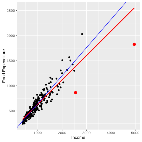
Figure 6.1: LAD vs OLS in R
[out] # A tibble: 6 × 2
[out]   income foodexp
[out]    <dbl>   <dbl>
[out] 1   420.    256.
[out] 2   541.    311.
[out] 3   901.    486.
[out] 4   639.    403.
[out] 5   751.    496.
[out] 6   946.    634.
Because of the sensitivity of the OLS regression to outliers, the OLS red line has been pulled down by the two red points. Whereas, the LAD blue line represents better the data.
We first move the data to python
if 'engel_py' not in globals():
  engel_py=r.engel
#import pandas as pd
#engel_py = pd.read_csv('engel.csv')
In Python we will use the statsmodels package:
import statsmodels.formula.api as smf

mod_reg_py = smf.quantreg('foodexp~income', data=engel_py).fit(q=0.25)
mod_reg_py.summary()
[out] <class 'statsmodels.iolib.summary.Summary'>
[out] """
[out] QuantReg Regression Results
[out] ==============================================================================
[out] Dep. Variable: foodexp Pseudo R-squared: 0.5540
[out] Model: QuantReg Bandwidth: 62.66
[out] Method: Least Squares Sparsity: 256.2
[out] Date: Thu, 17 Sept 2026 No. Observations: 235
[out] Time: 11:13:41 Df Residuals: 233
[out] Df Model: 1
[out] ==============================================================================
[out] coef std err t P>|t| [0.025 0.975]
[out] ------------------------------------------------------------------------------
[out] Intercept 95.4835 18.471 5.169 0.000 59.092 131.875
[out] income 0.4741 0.017 27.310 0.000 0.440 0.508
[out] ==============================================================================
[out]
[out] The condition number is large, 2.38e+03. This might indicate that there are
[out] strong multicollinearity or other numerical problems.
[out] """import statsmodels.formula.api as smf
import matplotlib.pyplot as plt
outliers = engel_py[(engel_py.income > 2500) & (engel_py.foodexp < 2000)]
fig= plt.figure(figsize=(5,3))
ax=plt.axes()
# LAD model
mod_reg2_py = smf.quantreg('foodexp~income', data=engel_py).fit(q=0.5)
# OLS model
mod_ols_py = smf.ols('foodexp~income', data=engel_py).fit()
ax.scatter(engel_py.income, engel_py.foodexp, color='black', s=5)
ax.scatter(outliers.income, outliers.foodexp, color='red', s=20)
plt.xlabel("Income")
plt.ylabel("Foodexp")
ax.plot(engel_py.income, mod_reg2_py.predict(engel_py.income), color="blue")
ax.plot(engel_py.income, mod_ols_py.predict(engel_py.income), color="red")
plt.savefig("engel_data.png")
plt.clf()
plt.close()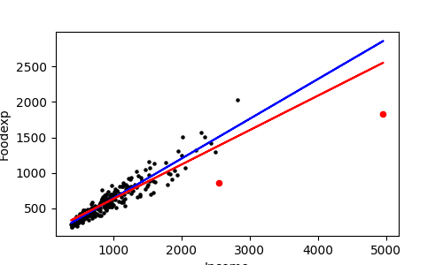
Figure 6.2: LAD vs OLS in Python