8.1 Concepts and definitions
The models of the previous chapters were built to be explained. We wrote a data generating process, we derived the properties of the estimators, and the coefficient \(\beta_1\) was read as the effect of a variable on another. The quality of such a model is judged on the plausibility of its assumptions as much as on its fit.
Machine learning starts from the other end. The question is no longer “what is the effect of \(x\) on \(y\)” but “how well can I predict \(y\) from \(x\) on data I have never seen”. The model is not required to be interpretable, only to generalize, and its quality is measured on observations that were kept aside during the estimation. This shift of objective explains everything that follows: the vocabulary, the algorithms, and above all the obsession with the separation between training and testing.
The two approaches are not opposed, they answer different questions. A model that predicts well may rest on a variable that has no causal role at all, and a correctly specified econometric model may predict poorly. Knowing which of the two questions we are asking is the first decision of any study.
8.1.1 Supervised learning: Regression and Classification
We speak of supervised learning when every observation of the training sample carries the answer we want to predict. The data are pairs \((x_i,y_i)\), where \(x_i\) is a vector of features and \(y_i\) the label, and the algorithm looks for a function \(f\) such that \(f(x_i)\) is as close as possible to \(y_i\).
The nature of the label splits the supervised problems into two families:
when \(y\) is a quantitative variable, we speak of regression, and the prediction is a number;
when \(y\) takes a finite number of values without any order, we speak of classification, and the prediction is a class.
The distinction is not a detail of vocabulary. It changes the function we fit, the loss we minimize and the way we measure the error, as the figure below shows.
In R:
set.seed(123)

# --- regression: a quantitative label
n <- 120
xr <- runif(n, 0, 10)
yr <- 2 + 1.2 * xr + rnorm(n, sd = 2)
dr <- data.frame(x = xr, y = yr)

p1 <- ggplot(dr, aes(x, y)) +
  geom_point(alpha = 0.6, colour = "grey30") +
  geom_smooth(method = "lm", se = FALSE, colour = "firebrick") +
  labs(title = "Regression", subtitle = "the label y is a number") +
  theme_minimal()

# --- classification: a qualitative label
g1 <- data.frame(x1 = rnorm(60, 2, 1), x2 = rnorm(60, 2, 1), class = "A")
g2 <- data.frame(x1 = rnorm(60, 5, 1), x2 = rnorm(60, 5, 1), class = "B")
dc <- rbind(g1, g2)

p2 <- ggplot(dc, aes(x1, x2, colour = class, shape = class)) +
  geom_point(alpha = 0.8) +
  geom_abline(intercept = 7, slope = -1, colour = "firebrick") +
  labs(title = "Classification", subtitle = "the label y is a class") +
  theme_minimal() + theme(legend.position = "bottom")

p1 + p2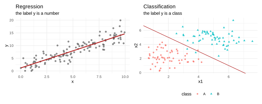
Figure 8.1: regression predicts a number, classification predicts a boundary
On the left the model answers with a value on the vertical axis. On the right it answers with a side of the line: everything below belongs to the first class, everything above to the second. The red line is called the decision boundary, and most of the classification algorithms differ only in the shape they allow that boundary to take.
In Python:
import numpy as np
import pandas as pd
import matplotlib.pyplot as plt

fig, ax = plt.subplots(1, 2, figsize=(9, 3.6))

ax[0].scatter(dr_py.x, dr_py.y, alpha=0.6, color="grey")
#> <matplotlib.collections.PathCollection object at 0x0000020E9CF00DA0>b = np.polyfit(dr_py.x, dr_py.y, 1)
xs = np.linspace(dr_py.x.min(), dr_py.x.max(), 50)
ax[0].plot(xs, np.polyval(b, xs), color="firebrick")#> [<matplotlib.lines.Line2D object at 0x0000020EB3A5E660>]#> Text(0.5, 1.0, 'Regression')for cl, mk in zip(["A", "B"], ["o", "^"]):
sub = dc_py[dc_py["class"] == cl]
ax[1].scatter(sub.x1, sub.x2, marker=mk, alpha=0.8, label=cl)#> <matplotlib.collections.PathCollection object at 0x0000020EB392FDD0>
#> <matplotlib.collections.PathCollection object at 0x0000020E9CE8D910>#> [<matplotlib.lines.Line2D object at 0x0000020EB3A5DD00>]#> Text(0.5, 1.0, 'Classification')#> <matplotlib.legend.Legend object at 0x0000020EB392FCE0>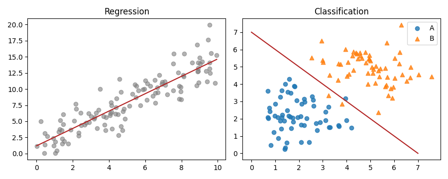
Figure 8.2: regression and classification in python
8.1.2 Multivariate regression
The regression above had a single output. When several quantitative labels must be predicted at the same time for each observation, we speak of multivariate regression, also called multi-output regression. A typical example is the prediction of the three components of a household budget, food, housing and transport, from the same set of characteristics.
Two strategies are possible. The simplest one fits an independent model for each output, which is easy but ignores the fact that the outputs are usually correlated. The second one estimates the outputs jointly and can exploit that correlation. The figure below shows the situation: the same predictor feeds two labels whose errors move together.
In R:
set.seed(123)
n <- 150
x <- runif(n, 0, 10)
shared <- rnorm(n, sd = 1.2)              # a common disturbance
y1 <- 1 + 1.0 * x + shared + rnorm(n, sd = 0.6)
y2 <- 4 - 0.7 * x + shared + rnorm(n, sd = 0.6)
dm <- data.frame(x, y1, y2)

q1 <- ggplot(dm, aes(x, y1)) + geom_point(alpha = .6, colour = "grey30") +
  geom_smooth(method = "lm", se = FALSE, colour = "firebrick") +
  labs(title = "first output") + theme_minimal()

q2 <- ggplot(dm, aes(x, y2)) + geom_point(alpha = .6, colour = "grey30") +
  geom_smooth(method = "lm", se = FALSE, colour = "steelblue") +
  labs(title = "second output") + theme_minimal()

res <- data.frame(e1 = residuals(lm(y1 ~ x)), e2 = residuals(lm(y2 ~ x)))
q3 <- ggplot(res, aes(e1, e2)) + geom_point(alpha = .6, colour = "grey30") +
  labs(title = "residuals of the two models",
       subtitle = paste("correlation =", round(cor(res$e1, res$e2), 2))) +
  theme_minimal()

q1 + q2 + q3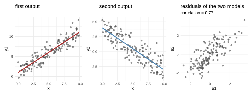
Figure 8.3: one predictor, two correlated outputs
The third panel is the important one. If the two sets of residuals were independent the cloud would be round, and fitting the two models separately would lose nothing. Here the cloud is clearly tilted, which means that knowing the error made on the first output tells us something about the error made on the second, and a joint estimation can exploit this information.
8.1.3 multi-label classfication
The same idea exists on the classification side, and the terminology deserves attention because three situations are easily confused:
binary classification: one label with two possible values, an email is spam or not;
multi-class classification: one label with more than two values, but exclusive, a handwritten digit is a \(3\) or a \(7\), never both;
multi-label classification: several labels at the same time, each of them present or absent, an article can be classified at once as economics, statistics and teaching.
The difference between the last two is the exclusivity. In the multi-class case the probabilities of the classes sum to one, in the multi-label case they do not, because the labels are answered independently.
In R:
set.seed(123)

# multi-class: three exclusive groups
mc <- rbind(
  data.frame(x1 = rnorm(50, 2, .7), x2 = rnorm(50, 2, .7), class = "A"),
  data.frame(x1 = rnorm(50, 5, .7), x2 = rnorm(50, 2, .7), class = "B"),
  data.frame(x1 = rnorm(50, 3.5, .7), x2 = rnorm(50, 5, .7), class = "C"))

m1 <- ggplot(mc, aes(x1, x2, colour = class, shape = class)) +
  geom_point(alpha = .8) +
  labs(title = "Multi-class", subtitle = "each point has exactly one label") +
  theme_minimal() + theme(legend.position = "bottom")

# multi-label: two labels that may overlap
set.seed(1)
ml <- data.frame(x1 = runif(150, 0, 6), x2 = runif(150, 0, 6))
ml$econ  <- ml$x1 > 3
ml$stat  <- ml$x2 > 3
ml$label <- with(ml, ifelse(econ & stat, "both",
                     ifelse(econ, "economics",
                     ifelse(stat, "statistics", "none"))))

m2 <- ggplot(ml, aes(x1, x2, colour = label)) +
  geom_point(alpha = .8) +
  geom_vline(xintercept = 3, linetype = 2) +
  geom_hline(yintercept = 3, linetype = 2) +
  labs(title = "Multi-label", subtitle = "a point may carry several labels") +
  theme_minimal() + theme(legend.position = "bottom")

m1 + m2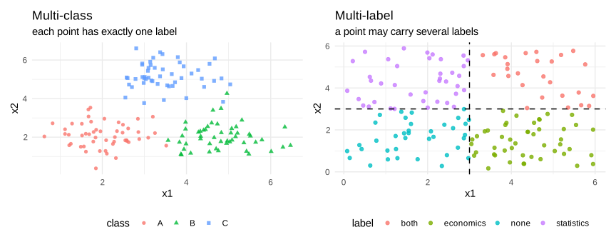
Figure 8.4: multi-class and multi-label are not the same problem
On the right the two dashed lines are two independent decision boundaries, one per label. The upper right quadrant carries both labels at once, which is impossible in the multi-class setting of the left panel.
8.1.4 Unsupervied learning: Clustring
In the unsupervised case the data contain no label at all. We only observe the vectors \(x_i\), and the algorithm is asked to find a structure in them by itself. Clustering is the most common task of this family: group the observations so that those inside a group resemble each other more than they resemble those of the other groups.
The difficulty, and it is a serious one, is that there is no right answer against which the result can be checked. With a label we could count the mistakes, here we cannot, and the evaluation relies on internal criteria that we describe in the section on metrics.
In R:
set.seed(123)
cl <- rbind(
  data.frame(x1 = rnorm(80, 2, .8), x2 = rnorm(80, 2, .8), truth = "1"),
  data.frame(x1 = rnorm(80, 6, .8), x2 = rnorm(80, 3, .8), truth = "2"),
  data.frame(x1 = rnorm(80, 4, .8), x2 = rnorm(80, 6.5, .8), truth = "3"))

u1 <- ggplot(cl, aes(x1, x2)) + geom_point(alpha = .7, colour = "grey30") +
  labs(title = "what the algorithm sees", subtitle = "no label") +
  theme_minimal()

km <- kmeans(cl[, 1:2], centers = 3, nstart = 20)
cl$found <- factor(km$cluster)

u2 <- ggplot(cl, aes(x1, x2, colour = found)) + geom_point(alpha = .8) +
  geom_point(data = as.data.frame(km$centers), aes(x1, x2),
             colour = "black", size = 4, shape = 4, inherit.aes = FALSE) +
  labs(title = "what it finds", subtitle = "three groups and their centres") +
  theme_minimal() + theme(legend.position = "bottom")

u1 + u2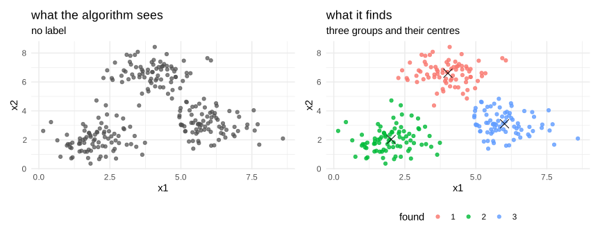
Figure 8.5: the same data, with and without the labels
The algorithm has recovered the three groups without ever being told that they existed. Note however that the numbers attached to the clusters are arbitrary: nothing guarantees that the cluster called \(1\) corresponds to the group that we simulated first, and this is why comparing a clustering to a known truth requires the special indices described later.
8.1.5 Semi supervised learning
Between the two previous situations lies a case that is very common in practice: a small number of labelled observations and a large number of unlabelled ones. Labelling is often expensive, because it requires a human expert, while collecting raw data is cheap.
Semi-supervised learning uses both. The intuition is that the unlabelled points reveal the shape of the data, and that the decision boundary should preferably pass through the empty regions rather than cut across a dense group. The figure below makes the argument visible.
In R:
set.seed(42)
ss <- rbind(
  data.frame(x1 = rnorm(100, 2, .8), x2 = rnorm(100, 2, .8), truth = "A"),
  data.frame(x1 = rnorm(100, 5, .8), x2 = rnorm(100, 5, .8), truth = "B"))

# only four points are labelled
lab_idx <- c(1, 2, 101, 102)
ss$known <- "unlabelled"
ss$known[lab_idx] <- ss$truth[lab_idx]

s1 <- ggplot(subset(ss, known != "unlabelled"), aes(x1, x2, colour = known)) +
  geom_point(size = 3) +
  xlim(range(ss$x1)) + ylim(range(ss$x2)) +
  labs(title = "only the labelled points", subtitle = "many boundaries are possible") +
  theme_minimal() + theme(legend.position = "bottom")

s2 <- ggplot(ss, aes(x1, x2)) +
  geom_point(data = subset(ss, known == "unlabelled"),
             colour = "grey75", alpha = .7) +
  geom_point(data = subset(ss, known != "unlabelled"),
             aes(colour = known), size = 3) +
  geom_abline(intercept = 7, slope = -1, colour = "firebrick") +
  labs(title = "with the unlabelled points",
       subtitle = "the empty corridor suggests the boundary") +
  theme_minimal() + theme(legend.position = "bottom")

s1 + s2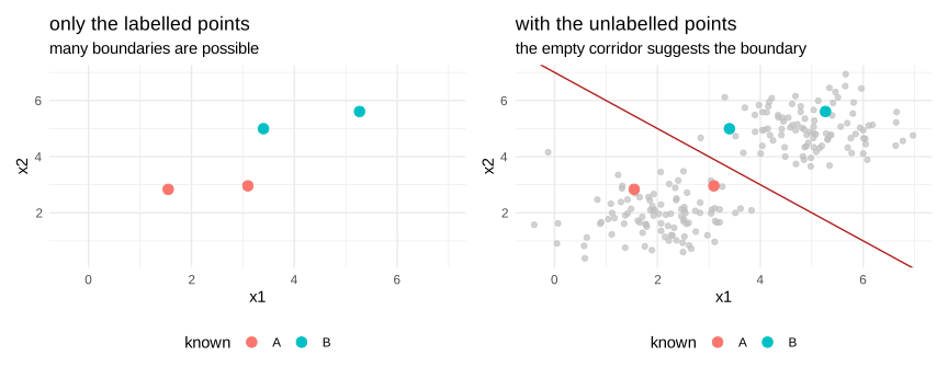
Figure 8.6: the unlabelled points change where the boundary should go
With four labelled points only, an infinity of boundaries separate them equally well. Once the grey cloud is added, one position becomes far more reasonable than the others, namely the empty corridor between the two groups. This is exactly the information that semi-supervised methods exploit.
8.1.6 The loss function and decision function
Fitting a model means choosing, inside a family of functions, the one that makes the fewest mistakes. To do that we need to say what a mistake costs, and this is the role of the loss function \(L(y,\hat y)\), which attaches a number to the gap between the observed value and the predicted one. The algorithm then minimizes the average loss on the training sample, called the empirical risk:
\[\begin{equation} R_{emp}(f)=\frac{1}{n}\sum_{i=1}^{n}L\big(y_i,f(x_i)\big) \tag{8.1} \end{equation}\]
Different losses give different models on the very same data, because they disagree on how severely a large error should be punished. For regression the two classical choices are the quadratic loss and the absolute loss, and the Huber loss is a compromise between them.
In R:
e <- seq(-3, 3, length.out = 400)
huber <- function(e, d = 1) ifelse(abs(e) <= d, 0.5 * e^2, d * (abs(e) - 0.5 * d))

dl <- rbind(
  data.frame(e, loss = e^2,        type = "quadratic"),
  data.frame(e, loss = abs(e),     type = "absolute"),
  data.frame(e, loss = huber(e),   type = "Huber"))

ggplot(dl, aes(e, loss, colour = type)) + geom_line(linewidth = 1) +
  labs(x = "error  y - yhat", y = "loss",
       title = "the loss decides how much a large error costs") +
  theme_minimal()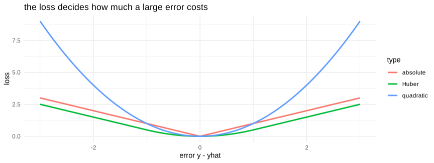
Figure 8.7: three losses for regression, as a function of the error
The quadratic loss grows very fast, so a single outlier can dominate the whole sum and pull the fitted model towards it. The absolute loss grows linearly and is therefore far more robust, at the price of a non differentiable point at zero. The Huber loss is quadratic near zero and linear far from it, which keeps the good behaviour of both.
For classification the prediction is usually not a class directly, but a decision function \(g(x)\), a real number whose sign gives the class and whose magnitude expresses the confidence. The losses are then written as functions of the quantity \(y\cdot g(x)\), called the margin, which is positive when the prediction is correct.
m <- seq(-3, 3, length.out = 400)
dl2 <- rbind(
  data.frame(m, loss = as.numeric(m <= 0),          type = "0-1 loss"),
  data.frame(m, loss = pmax(0, 1 - m),              type = "hinge (SVM)"),
  data.frame(m, loss = log(1 + exp(-m)) / log(2),   type = "logistic"))

ggplot(dl2, aes(m, loss, colour = type)) + geom_line(linewidth = 1) +
  geom_vline(xintercept = 0, linetype = 2, colour = "grey50") +
  labs(x = "margin  y * g(x)", y = "loss",
       title = "the margin is positive when the prediction is correct") +
  theme_minimal()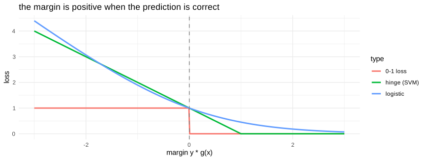
Figure 8.8: three losses for classification, as a function of the margin
The \(0-1\) loss is the one we really care about, since it simply counts the mistakes, but it is flat everywhere and jumps at zero, so no gradient can be used to minimize it. The hinge loss and the logistic loss are convex upper bounds of it, differentiable enough to be optimized, and they are what the support vector machine and the logistic regression actually minimize.
8.1.7 Training and Testing
Here lies the central rule of the whole discipline. The error measured on the data that served to fit the model is not an estimate of the error we will make on new data, it is systematically too optimistic, because the model has had the opportunity to adapt to the particular noise of that sample.
The sample is therefore split. The training set is used to fit, the test set is used once, at the very end, to obtain an honest measure of the performance. When several models or several tuning values must be compared, a third block is needed, the validation set, or better, cross validation: the training set is cut into \(k\) folds, the model is fitted \(k\) times, each time leaving one fold aside to evaluate it, and the \(k\) results are averaged.
In R:
# a simple picture of the split
split_df <- data.frame(
  part = factor(c("training", "validation", "test"),
                levels = c("training", "validation", "test")),
  start = c(0, 60, 80), end = c(60, 80, 100))

t1 <- ggplot(split_df) +
  geom_rect(aes(xmin = start, xmax = end, ymin = 0, ymax = 1, fill = part),
            colour = "white") +
  labs(title = "one split of the sample", x = "% of the observations", y = "") +
  theme_minimal() + theme(axis.text.y = element_blank(), legend.position = "bottom")

# the k folds
k <- 5
folds <- do.call(rbind, lapply(1:k, function(i) {
  data.frame(rep = paste("fold", i), start = seq(0, 80, by = 20),
             end = seq(20, 100, by = 20),
             role = ifelse(seq_len(5) == i, "evaluation", "fitting"))
}))

t2 <- ggplot(folds) +
  geom_rect(aes(xmin = start, xmax = end, ymin = 0, ymax = .8, fill = role),
            colour = "white") +
  facet_wrap(~ rep, ncol = 1) +
  labs(title = "5-fold cross validation", x = "% of the observations", y = "") +
  theme_minimal() + theme(axis.text.y = element_blank(), legend.position = "bottom")

t1 + t2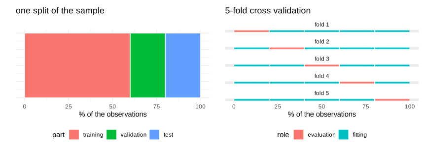
Figure 8.9: the split of the sample and the k-fold cross validation
Each row of the right panel is one of the five fits. The block used for the evaluation moves from left to right, so that every observation is used once for evaluation and four times for fitting, and the final score is the average of the five.
The test set must be touched only once. If we look at it, change the model, and look again, it progressively becomes a second training set and its error becomes optimistic in its turn. This form of leakage is silent and very frequent, and it is the reason why the validation set, or the cross validation, exists at all.
8.1.8 underfiting and overfiting problem
We can now state the central difficulty. A model that is too simple cannot represent the relation, and it makes large errors everywhere, on the training set as well as on the test set: we say that it underfits, and that it has a high bias. A model that is too flexible follows the training points almost exactly, including their noise, and it fails on any new point: it overfits, and it has a high variance.
The expected error of a prediction decomposes into three terms that make this trade-off explicit:
\[\begin{equation} E\big[(y-\hat f(x))^2\big]=\underbrace{\big(E[\hat f(x)]-f(x)\big)^2}_{bias^2}+\underbrace{Var\big(\hat f(x)\big)}_{variance}+\underbrace{\sigma^2}_{irreducible} \tag{8.2} \end{equation}\]
The last term is the noise of the data and no model can remove it. The first two move in opposite directions when the complexity increases, and the whole art consists in finding the point where their sum is smallest.
In R:
set.seed(123)
n <- 40
x <- sort(runif(n, 0, 1))
f_true <- function(x) sin(2 * pi * x)
y <- f_true(x) + rnorm(n, sd = 0.3)
dat <- data.frame(x, y)
grid <- data.frame(x = seq(0, 1, length.out = 300))

fit_plot <- function(deg, title) {
  fit <- lm(y ~ poly(x, deg), data = dat)
  grid$pred <- predict(fit, newdata = grid)
  ggplot(dat, aes(x, y)) +
    geom_point(alpha = .7, colour = "grey30") +
    stat_function(fun = f_true, colour = "grey60", linetype = 2) +
    geom_line(data = grid, aes(x, pred), colour = "firebrick", linewidth = 1) +
    labs(title = title) + ylim(-2.2, 2.2) + theme_minimal()
}

fit_plot(1, "degree 1 : underfitting") +
  fit_plot(5, "degree 5 : about right") +
  fit_plot(20, "degree 20 : overfitting")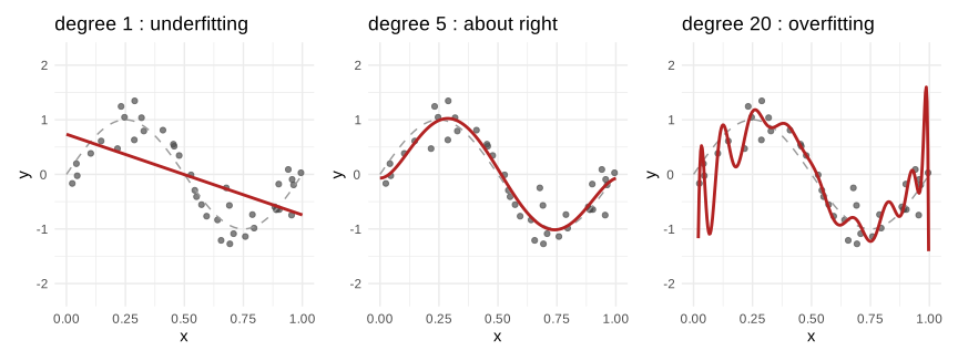
Figure 8.10: the same data fitted with three degrees of flexibility
The dashed grey curve is the true relation. On the left the straight line is far from it everywhere. On the right the curve passes very close to the points but oscillates wildly between them, and those oscillations are pure noise: on a new sample they would be different.
The consequence is best seen by plotting the two errors against the complexity.
set.seed(123)
x_tr <- sort(runif(60, 0, 1)); y_tr <- f_true(x_tr) + rnorm(60, sd = .3)
x_te <- sort(runif(300, 0, 1)); y_te <- f_true(x_te) + rnorm(300, sd = .3)
tr <- data.frame(x = x_tr, y = y_tr); te <- data.frame(x = x_te, y = y_te)

degs <- 1:18
err <- do.call(rbind, lapply(degs, function(d) {
  fit <- lm(y ~ poly(x, d), data = tr)
  data.frame(degree = d,
             train = mean((tr$y - predict(fit))^2),
             test  = mean((te$y - predict(fit, newdata = te))^2))
}))

err_long <- rbind(data.frame(degree = err$degree, mse = err$train, set = "training"),
                  data.frame(degree = err$degree, mse = err$test,  set = "test"))

ggplot(err_long, aes(degree, mse, colour = set)) +
  geom_line(linewidth = 1) + geom_point() +
  scale_y_log10() +
  geom_vline(xintercept = degs[which.min(err$test)], linetype = 2, colour = "grey40") +
  labs(title = "the U shape of the test error",
       x = "degree of the polynomial", y = "mean squared error (log scale)") +
  theme_minimal()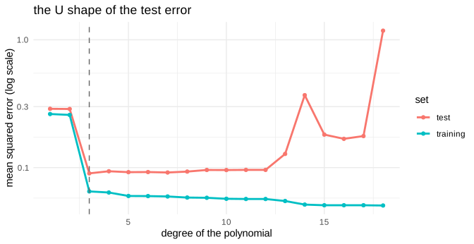
Figure 8.11: training error always decreases, test error does not
This picture is the one to keep in mind. The training error, in one colour, decreases monotonically: adding flexibility can only improve the fit on the points that were used to fit. The test error, in the other, first decreases because the model captures more of the real relation, then increases because it starts capturing the noise. The dashed line marks the best compromise, and everything to its right is overfitting.
In Python:
The same experiment is written with scikit-learn, which chains the polynomial expansion and the regression in a pipeline.
from sklearn.pipeline import make_pipeline
from sklearn.preprocessing import PolynomialFeatures
from sklearn.linear_model import LinearRegression
from sklearn.metrics import mean_squared_error

rng = np.random.default_rng(123)
f_true_py = lambda z: np.sin(2 * np.pi * z)

x_tr_py = np.sort(rng.uniform(0, 1, 60)); y_tr_py = f_true_py(x_tr_py) + rng.normal(0, .3, 60)
x_te_py = np.sort(rng.uniform(0, 1, 300)); y_te_py = f_true_py(x_te_py) + rng.normal(0, .3, 300)

degrees = range(1, 19)
tr_err, te_err = [], []
for d in degrees:
    mod = make_pipeline(PolynomialFeatures(d), LinearRegression())
    mod.fit(x_tr_py.reshape(-1, 1), y_tr_py)
    tr_err.append(mean_squared_error(y_tr_py, mod.predict(x_tr_py.reshape(-1, 1))))
    te_err.append(mean_squared_error(y_te_py, mod.predict(x_te_py.reshape(-1, 1))))
#> Pipeline(steps=[('polynomialfeatures', PolynomialFeatures(degree=1)),
#> ('linearregression', LinearRegression())])
#> Pipeline(steps=[('polynomialfeatures', PolynomialFeatures()),
#> ('linearregression', LinearRegression())])
#> Pipeline(steps=[('polynomialfeatures', PolynomialFeatures(degree=3)),
#> ('linearregression', LinearRegression())])
#> Pipeline(steps=[('polynomialfeatures', PolynomialFeatures(degree=4)),
#> ('linearregression', LinearRegression())])
#> Pipeline(steps=[('polynomialfeatures', PolynomialFeatures(degree=5)),
#> ('linearregression', LinearRegression())])
#> Pipeline(steps=[('polynomialfeatures', PolynomialFeatures(degree=6)),
#> ('linearregression', LinearRegression())])
#> Pipeline(steps=[('polynomialfeatures', PolynomialFeatures(degree=7)),
#> ('linearregression', LinearRegression())])
#> Pipeline(steps=[('polynomialfeatures', PolynomialFeatures(degree=8)),
#> ('linearregression', LinearRegression())])
#> Pipeline(steps=[('polynomialfeatures', PolynomialFeatures(degree=9)),
#> ('linearregression', LinearRegression())])
#> Pipeline(steps=[('polynomialfeatures', PolynomialFeatures(degree=10)),
#> ('linearregression', LinearRegression())])
#> Pipeline(steps=[('polynomialfeatures', PolynomialFeatures(degree=11)),
#> ('linearregression', LinearRegression())])
#> Pipeline(steps=[('polynomialfeatures', PolynomialFeatures(degree=12)),
#> ('linearregression', LinearRegression())])
#> Pipeline(steps=[('polynomialfeatures', PolynomialFeatures(degree=13)),
#> ('linearregression', LinearRegression())])
#> Pipeline(steps=[('polynomialfeatures', PolynomialFeatures(degree=14)),
#> ('linearregression', LinearRegression())])
#> Pipeline(steps=[('polynomialfeatures', PolynomialFeatures(degree=15)),
#> ('linearregression', LinearRegression())])
#> Pipeline(steps=[('polynomialfeatures', PolynomialFeatures(degree=16)),
#> ('linearregression', LinearRegression())])
#> Pipeline(steps=[('polynomialfeatures', PolynomialFeatures(degree=17)),
#> ('linearregression', LinearRegression())])
#> Pipeline(steps=[('polynomialfeatures', PolynomialFeatures(degree=18)),
#> ('linearregression', LinearRegression())])#> <Figure size 600x340 with 0 Axes>#> [<matplotlib.lines.Line2D object at 0x0000020EB3ADB0E0>]#> [<matplotlib.lines.Line2D object at 0x0000020EB38C82C0>]#> <matplotlib.lines.Line2D object at 0x0000020E9CE44FE0>#> Text(0.5, 0, 'degree of the polynomial')
#> Text(0, 0.5, 'mean squared error')#> <matplotlib.legend.Legend object at 0x0000020EB38CAF00>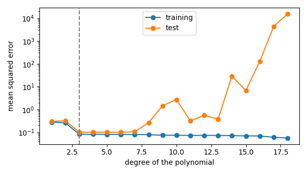
Figure 8.12: bias variance trade-off in python
The curve has the same shape, and the minimum falls at a comparable degree. The exact position moves a little from one simulation to another, which is itself a reminder that the choice of the complexity is estimated, and therefore uncertain.
A last way of looking at the same phenomenon is the learning curve, which fixes the model and varies the size of the training sample. It answers a practical question that the previous plot does not: would collecting more data help?
In R:
set.seed(123)
# the smallest sample must stay larger than the degree of the polynomial,
# otherwise the fit is not defined
sizes <- seq(25, 200, by = 10)
big_te <- data.frame(x = runif(500, 0, 1)); big_te$y <- f_true(big_te$x) + rnorm(500, sd = .3)

learn <- function(deg) {
  do.call(rbind, lapply(sizes, function(m) {
    xs <- runif(m, 0, 1); ys <- f_true(xs) + rnorm(m, sd = .3)
    d  <- data.frame(x = xs, y = ys)
    fit <- lm(y ~ poly(x, deg), data = d)
    data.frame(size = m, degree = paste("degree", deg),
               train = mean((d$y - predict(fit))^2),
               test  = mean((big_te$y - predict(fit, newdata = big_te))^2))
  }))
}

lc <- rbind(learn(1), learn(15))
lc_long <- rbind(data.frame(lc[, c("size", "degree")], mse = lc$train, set = "training"),
                 data.frame(lc[, c("size", "degree")], mse = lc$test,  set = "test"))

ggplot(lc_long, aes(size, mse, colour = set)) +
  geom_line(linewidth = .9) +
  facet_wrap(~ degree, scales = "free_y") +
  labs(title = "learning curves", x = "size of the training sample",
       y = "mean squared error") +
  theme_minimal()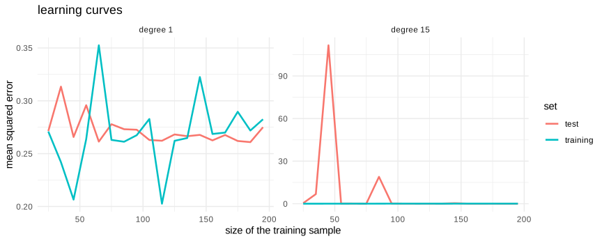
Figure 8.13: learning curves for a model that underfits and one that overfits
The two panels tell very different stories. On the left, with a model that underfits, the two curves meet quickly at a high level and stay flat: more data will not help, the model itself is too rigid and must be made more flexible. On the right, with a model that overfits, a wide gap separates the two curves and it narrows as the sample grows: here more data is exactly what is needed. Reading this gap before deciding what to do next saves a lot of wasted effort.
8.1.9 Metrics and scores
Once a model is fitted we must say how good it is, and this requires a number. The choice of that number is not a technical formality: it defines what “good” means for the problem at hand, and two metrics can rank the same two models in opposite orders. A metric that averages squared errors will prefer a model that never makes a large mistake, one that averages absolute errors will prefer a model that is right most of the time even if it is occasionally very wrong. Choosing the metric is therefore part of the modelling, and it should be decided before looking at the results, not after.
We distinguish the metrics by the type of problem: regression, classification, and clustering.
8.1.9.1 Metrics for regression
All the metrics below compare the observed values \(y_i\) to the predictions \(\hat y_i\) over \(n\) observations.
mean squared error:
\[\begin{equation} MSE=\frac{1}{n}\sum_{i=1}^{n}(y_i-\hat y_i)^2 \tag{8.3} \end{equation}\]
The reference metric, and the one that the ordinary least squares minimize. Because the errors are squared, a single large mistake weighs as much as many small ones, so the \(MSE\) is very sensitive to outliers. Its unit is the square of the unit of \(y\), which is why its root, the \(RMSE\), is often preferred for reporting.
mean absolute error:
\[\begin{equation} MAE=\frac{1}{n}\sum_{i=1}^{n}\lvert y_i-\hat y_i\rvert \tag{8.4} \end{equation}\]
The average size of the mistake, expressed in the unit of \(y\), which makes it easy to explain to a non specialist. It treats all the errors proportionally and is therefore much more robust than the \(MSE\).
mean squared log error:
\[\begin{equation} MSLE=\frac{1}{n}\sum_{i=1}^{n}\big(\ln(1+y_i)-\ln(1+\hat y_i)\big)^2 \tag{8.5} \end{equation}\]
Used when the target spans several orders of magnitude, or when we care about the relative error rather than the absolute one. Being under by \(10\) on a value of \(20\) is penalized much more than being under by \(10\) on a value of \(10000\). It requires positive values, and it penalizes under-prediction more than over-prediction.
median absolute error:
\[\begin{equation} MedAE=median\big(\lvert y_1-\hat y_1\rvert,...,\lvert y_n-\hat y_n\rvert\big) \tag{8.6} \end{equation}\]
The most robust of the family. A group of outliers, as long as it stays a minority, does not move the median at all. The price is that it ignores the size of the large errors completely, which is not always desirable.
R square:
\[\begin{equation} R^2=1-\frac{\sum_{i=1}^{n}(y_i-\hat y_i)^2}{\sum_{i=1}^{n}(y_i-\bar y)^2} \tag{8.7} \end{equation}\]
The share of the variance explained by the model, and the only metric of this list that is unitless and therefore comparable across problems. Contrary to the econometric context, where it is computed on the sample that served to fit, here it is evaluated on the test set, and it may perfectly well be negative if the model predicts worse than the simple mean.
mean absolute percentage error:
\[\begin{equation} MAPE=\frac{100}{n}\sum_{i=1}^{n}\left\lvert\frac{y_i-\hat y_i}{y_i}\right\rvert \tag{8.8} \end{equation}\]
Expresses the error as a percentage of the observed value, which is convenient for forecasting. It has two well known defects: it explodes when \(y_i\) is close to zero, and it is asymmetric, since an over-prediction can cost at most \(100\%\) while an under-prediction is unbounded.
mean poisson deviance:
\[\begin{equation} D_{Poisson}=\frac{2}{n}\sum_{i=1}^{n}\left(y_i\ln\frac{y_i}{\hat y_i}-(y_i-\hat y_i)\right) \tag{8.9} \end{equation}\]
The right metric when the target is a count, such as a number of claims or of visits. It is the deviance of the Poisson model met in the chapter on non linear models, and it accounts for the fact that the variance of a count grows with its mean.
mean gamma deviance:
\[\begin{equation} D_{Gamma}=\frac{2}{n}\sum_{i=1}^{n}\left(\ln\frac{\hat y_i}{y_i}+\frac{y_i}{\hat y_i}-1\right) \tag{8.10} \end{equation}\]
The counterpart for positive continuous targets whose variance grows with the square of the mean, typically an amount of money. Both deviances belong to the same family, the Tweedie deviances, indexed by the power that links the variance to the mean.
The following experiment shows why the choice matters. We take a well behaved sample, add a handful of outliers, and watch how each metric reacts.
In R:
set.seed(123)
n <- 200
x <- runif(n, 1, 20)
y <- 5 + 2 * x + rnorm(n, sd = 3)

# a copy with a few strong outliers
y_out <- y
idx <- sample(n, 8)
y_out[idx] <- y_out[idx] + 60

fit_clean <- lm(y ~ x)
fit_out   <- lm(y_out ~ x)

d1 <- data.frame(x, y, fitted = fitted(fit_clean), kind = "without outliers")
d2 <- data.frame(x, y = y_out, fitted = fitted(fit_out), kind = "with outliers")
dd <- rbind(d1, d2)

ggplot(dd, aes(x, y)) +
  geom_point(alpha = .6, colour = "grey30") +
  geom_line(aes(y = fitted), colour = "firebrick", linewidth = 1) +
  facet_wrap(~ kind) +
  labs(title = "eight outliers are enough to tilt the line") +
  theme_minimal()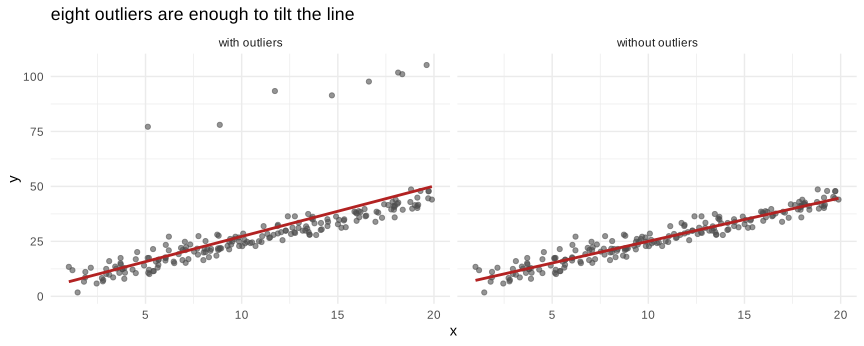
Figure 8.14: the same predictions judged by different metrics
metrics_reg <- function(y, yhat) {
  e <- y - yhat
  data.frame(
    MSE   = mean(e^2),
    RMSE  = sqrt(mean(e^2)),
    MAE   = mean(abs(e)),
    MedAE = median(abs(e)),
    MAPE  = 100 * mean(abs(e / y)),
    R2    = 1 - sum(e^2) / sum((y - mean(y))^2)
  )
}

comp <- rbind(
  cbind(data = "without outliers", metrics_reg(y, fitted(fit_clean))),
  cbind(data = "with outliers",    metrics_reg(y_out, fitted(fit_out)))
)| data | MSE | RMSE | MAE | MedAE | MAPE | R2 |
|---|---|---|---|---|---|---|
| without outliers | 8.289 | 2.879 | 2.284 | 1.834 | 13.010 | 0.927 |
| with outliers | 143.801 | 11.992 | 5.592 | 3.279 | 18.997 | 0.496 |
The lesson is in the ratios rather than in the levels. Between the two rows the \(MSE\) is multiplied by roughly seventeen, the \(MAE\) by less than three, and the median absolute error by less than two: the order of sensitivity is exactly the one the formulas predict. Note that the robust metrics are reduced, not immune. The eight outliers do not only add eight large residuals, they also tilt the fitted line itself, and a tilted line moves every residual, including those of the well behaved points. No metric can protect a model against a fit that has already been distorted, which is why the outliers must be dealt with at the estimation stage, through a robust loss, and not merely at the evaluation stage. If the outliers are genuine observations that we must predict well, the \(MSE\) is the honest metric. If they are recording errors, optimizing the \(MSE\) will drag the model towards them and the \(MAE\) is the safer choice.
In Python:
The module sklearn.metrics provides all of them under explicit names.
if 'y_ml_py' not in globals():
  y_ml_py = r.y
if 'yhat_ml_py' not in globals():
  yhat_ml_py = r.d1["fitted"]
from sklearn.metrics import (mean_squared_error, mean_absolute_error,
                             median_absolute_error, r2_score,
                             mean_absolute_percentage_error)

yv = np.asarray(y_ml_py, dtype=float)
pv = np.asarray(yhat_ml_py, dtype=float)

reg_metrics_py = pd.DataFrame([{
    "MSE":   round(mean_squared_error(yv, pv), 3),
    "RMSE":  round(float(np.sqrt(mean_squared_error(yv, pv))), 3),
    "MAE":   round(mean_absolute_error(yv, pv), 3),
    "MedAE": round(median_absolute_error(yv, pv), 3),
    "MAPE":  round(100 * mean_absolute_percentage_error(yv, pv), 3),
    "R2":    round(r2_score(yv, pv), 3)
}])| MSE | RMSE | MAE | MedAE | MAPE | R2 |
|---|---|---|---|---|---|
| 8.289 | 2.879 | 2.284 | 1.834 | 13.01 | 0.927 |
8.1.9.2 Metrics for classification
Everything in classification starts from one table, so we describe it first even though the outline places it further down.
confusion matrix:
The confusion matrix cross-tabulates the observed class against the predicted one. For a binary problem it has four cells, and the whole vocabulary of this section is built on them:
\[\begin{equation} \begin{matrix} & \hat y=1 & \hat y=0 \\ y=1 & TP & FN \\ y=0 & FP & TN \end{matrix} \tag{8.11} \end{equation}\]
where \(TP\) counts the true positives, \(FN\) the false negatives, \(FP\) the false positives and \(TN\) the true negatives. The two types of error are not interchangeable: refusing a loan to a solvent client and granting one to an insolvent client have very different costs, and a single number can rarely represent both.
accuracy:
\[\begin{equation} Accuracy=\frac{TP+TN}{TP+TN+FP+FN} \tag{8.12} \end{equation}\]
The share of correct predictions. It is the most intuitive metric and the most dangerous one, because on an unbalanced problem it is maximized by the model that always predicts the majority class. If one per cent of the transactions are fraudulent, a model that never detects any fraud is right ninety nine per cent of the time.
Precision:
\[\begin{equation} Precision=\frac{TP}{TP+FP} \tag{8.13} \end{equation}\]
Among the observations declared positive, the share that really is. It answers the question “when the model raises an alarm, how often should I believe it”.
recall:
\[\begin{equation} Recall=\frac{TP}{TP+FN} \tag{8.14} \end{equation}\]
Among the observations that really are positive, the share that the model found. It answers “of everything I should have caught, how much did I catch”. Precision and recall move in opposite directions: lowering the threshold catches more positives but raises the number of false alarms.
F measures:
\[\begin{equation} F_\beta=(1+\beta^2)\frac{Precision\times Recall}{\beta^2 Precision+Recall} \tag{8.15} \end{equation}\]
Their harmonic mean, weighted by \(\beta\). With \(\beta=1\) we obtain the usual \(F_1\), which treats them symmetrically. Taking \(\beta>1\) gives more weight to the recall, which is what we want when missing a positive is the costly mistake, for instance in medical screening.
receiver operating characteristic curve ROC:
Most classifiers return a probability, and the class follows from a threshold. Rather than fixing one threshold, the ROC curve plots the true positive rate against the false positive rate as the threshold sweeps from one to zero. The area under this curve, the \(AUC\), summarizes the whole family of thresholds in one number, and it has a clean interpretation: it is the probability that a randomly chosen positive receives a higher score than a randomly chosen negative. A value of \(0.5\) means the model is worthless, \(1\) means perfect separation.
balanced accuracy:
\[\begin{equation} BalancedAccuracy=\frac{1}{2}\left(\frac{TP}{TP+FN}+\frac{TN}{TN+FP}\right) \tag{8.16} \end{equation}\]
The mean of the recalls of the two classes, which repairs the main defect of the accuracy on unbalanced data: the trivial model that always answers the majority class obtains exactly \(0.5\).
top k-accuracy:
An observation is counted as correct if its true class appears among the \(k\) classes judged most probable by the model. It is used when the number of classes is large and when the model is a first filter proposed to a human, rather than a final decision.
Cohen’s kappa:
\[\begin{equation} \kappa=\frac{p_o-p_e}{1-p_e} \tag{8.17} \end{equation}\]
where \(p_o\) is the observed accuracy and \(p_e\) the accuracy that pure chance would obtain given the marginal frequencies. It measures the agreement corrected for chance, and it is null for a model that does no better than random guessing.
log loss:
\[\begin{equation} LogLoss=-\frac{1}{n}\sum_{i=1}^{n}\Big(y_i\ln(\hat p_i)+(1-y_i)\ln(1-\hat p_i)\Big) \tag{8.18} \end{equation}\]
Unlike the previous metrics, it judges the probabilities and not the classes. It punishes confident mistakes very severely, since predicting a probability of \(0.01\) for an event that occurs sends the logarithm towards infinity. It is the loss that the logistic regression minimizes.
Brier score loss:
\[\begin{equation} Brier=\frac{1}{n}\sum_{i=1}^{n}(\hat p_i-y_i)^2 \tag{8.19} \end{equation}\]
The quadratic equivalent of the log loss on the probabilities. It is bounded between zero and one and punishes a confident mistake less brutally, which makes it more stable when a few probabilities are extreme.
Hamming distance:
The share of labels that are wrong, averaged over all the labels and all the observations. On a simple classification it coincides with one minus the accuracy, but its real use is in the multi-label setting described earlier, where each observation carries several labels and where a prediction can be partly right.
jaccard similarity:
\[\begin{equation} J=\frac{\lvert A\cap B\rvert}{\lvert A\cup B\rvert}=\frac{TP}{TP+FP+FN} \tag{8.20} \end{equation}\]
The size of the intersection over the size of the union of the predicted and the true sets of labels. Contrary to the accuracy it ignores the true negatives entirely, which is an advantage when the absence of a label is the uninformative case.
hinge loss:
\[\begin{equation} L_{hinge}=\frac{1}{n}\sum_{i=1}^{n}\max\big(0,1-y_i g(x_i)\big) \tag{8.21} \end{equation}\]
Already plotted in the section on the loss functions. It is zero as soon as the point is on the right side and far enough from the boundary, which is what gives the support vector machine its margin.
Matthews correlation coefficient:
\[\begin{equation} MCC=\frac{TP\times TN-FP\times FN}{\sqrt{(TP+FP)(TP+FN)(TN+FP)(TN+FN)}} \tag{8.22} \end{equation}\]
A correlation coefficient between the observed and the predicted classes, lying between \(-1\) and \(1\). It is the only metric of this list that uses the four cells of the confusion matrix in a balanced way, and it is therefore the most reliable single number on unbalanced problems.
Zero one loss:
The share of misclassified observations, that is exactly one minus the accuracy. It is the loss we would like to minimize directly, but as we saw it is not differentiable, so the algorithms minimize a convex surrogate instead.
Let us now compute these quantities on a deliberately unbalanced problem, where the differences between them become visible.
In R:
set.seed(123)
n <- 1000
x1 <- rnorm(n); x2 <- rnorm(n)
# only about 12 per cent of positives
lin <- -2.2 + 1.5 * x1 + 1.2 * x2
p   <- 1 / (1 + exp(-lin))
ycl <- rbinom(n, 1, p)

tr_idx <- sample(n, 700)
train <- data.frame(x1, x2, y = ycl)[tr_idx, ]
test  <- data.frame(x1, x2, y = ycl)[-tr_idx, ]

mod <- glm(y ~ x1 + x2, data = train, family = binomial)
prob <- predict(mod, newdata = test, type = "response")
pred <- as.integer(prob > 0.5)

cm <- table(observed = test$y, predicted = pred)

cm_df <- as.data.frame(cm)
ggplot(cm_df, aes(predicted, observed, fill = Freq)) +
  geom_tile(colour = "white") +
  geom_text(aes(label = Freq), size = 5) +
  scale_fill_gradient(low = "white", high = "steelblue") +
  labs(title = "confusion matrix", subtitle = "threshold = 0.5") +
  theme_minimal()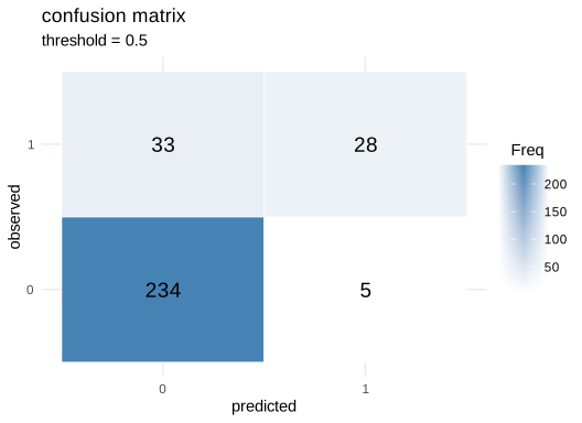
Figure 8.15: confusion matrix of a logistic model on unbalanced data
TP <- cm["1", "1"]; TN <- cm["0", "0"]
FP <- cm["0", "1"]; FN <- cm["1", "0"]

prec <- TP / (TP + FP); rec <- TP / (TP + FN)
acc  <- (TP + TN) / sum(cm)
po   <- acc
pe   <- sum(rowSums(cm) * colSums(cm)) / sum(cm)^2

class_metrics <- data.frame(
  accuracy          = acc,
  balanced_accuracy = 0.5 * (rec + TN / (TN + FP)),
  precision         = prec,
  recall            = rec,
  F1                = 2 * prec * rec / (prec + rec),
  kappa             = (po - pe) / (1 - pe),
  MCC               = (TP * TN - FP * FN) /
                       sqrt((TP + FP) * (TP + FN) * (TN + FP) * (TN + FN)),
  log_loss          = -mean(test$y * log(prob) + (1 - test$y) * log(1 - prob)),
  brier             = mean((prob - test$y)^2)
)| value | |
|---|---|
| accuracy | 0.8733 |
| balanced_accuracy | 0.7190 |
| precision | 0.8485 |
| recall | 0.4590 |
| F1 | 0.5957 |
| kappa | 0.5284 |
| MCC | 0.5635 |
| log_loss | 0.2972 |
| brier | 0.0883 |
The accuracy looks flattering, and it is: the positives are rare, so predicting the negative class almost always is nearly free. The balanced accuracy, the \(F_1\), the kappa and the \(MCC\) are all clearly lower, and they are the numbers to report. This gap between a comfortable accuracy and much more modest companions is the standard signature of an unbalanced problem.
The threshold of \(0.5\) has nothing sacred about it. Moving it trades precision against recall, and the two curves below show the whole range of the compromise.
thr <- seq(0.01, 0.95, by = 0.01)
tradeoff <- do.call(rbind, lapply(thr, function(t) {
  pr <- as.integer(prob > t)
  tp <- sum(pr == 1 & test$y == 1); fp <- sum(pr == 1 & test$y == 0)
  fn <- sum(pr == 0 & test$y == 1); tn <- sum(pr == 0 & test$y == 0)
  data.frame(threshold = t,
             precision = ifelse(tp + fp == 0, NA, tp / (tp + fp)),
             recall    = tp / (tp + fn),
             tpr       = tp / (tp + fn),
             fpr       = fp / (fp + tn))
}))

pr_long <- rbind(
  data.frame(threshold = tradeoff$threshold, value = tradeoff$precision, metric = "precision"),
  data.frame(threshold = tradeoff$threshold, value = tradeoff$recall,    metric = "recall"))

r1 <- ggplot(pr_long, aes(threshold, value, colour = metric)) +
  geom_line(linewidth = 1) +
  geom_vline(xintercept = .5, linetype = 2, colour = "grey50") +
  labs(title = "precision and recall against the threshold") +
  theme_minimal() + theme(legend.position = "bottom")

auc <- with(tradeoff[order(tradeoff$fpr), ],
            sum(diff(c(0, fpr, 1)) * (c(0, tpr, 1)[-1] + c(0, tpr, 1)[-length(c(0, tpr, 1))]) / 2))

r2 <- ggplot(tradeoff, aes(fpr, tpr)) +
  geom_line(colour = "firebrick", linewidth = 1) +
  geom_abline(intercept = 0, slope = 1, linetype = 2, colour = "grey50") +
  labs(title = "ROC curve", subtitle = paste("AUC =", round(auc, 3)),
       x = "false positive rate", y = "true positive rate") +
  theme_minimal()

r1 + r2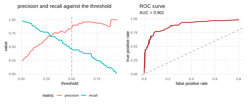
Figure 8.16: the threshold governs the compromise, and the ROC summarizes it
On the left, raising the threshold makes the model more demanding: it raises the precision and lowers the recall. The dashed line marks the default of \(0.5\), and nothing suggests that it is the best place to stand. On the right, the ROC curve gathers every threshold at once, and the diagonal is the model that answers at random. The further the curve bulges towards the upper left corner, the better the ranking produced by the model.
In Python:
if 'prob_py' not in globals():
  prob_py = r.prob
if 'ytest_py' not in globals():
  ytest_py = r.test["y"]
from sklearn.metrics import (roc_curve, roc_auc_score, precision_score,
recall_score, f1_score, accuracy_score,
balanced_accuracy_score, cohen_kappa_score,
matthews_corrcoef, log_loss, brier_score_loss)
pp = np.asarray(prob_py, dtype=float)
yy = np.asarray(ytest_py, dtype=int)
pc = (pp > 0.5).astype(int)
cls_py = pd.DataFrame([{
"accuracy": round(accuracy_score(yy, pc), 4),
"balanced_accuracy": round(balanced_accuracy_score(yy, pc), 4),
"precision": round(precision_score(yy, pc), 4),
"recall": round(recall_score(yy, pc), 4),
"F1": round(f1_score(yy, pc), 4),
"kappa": round(cohen_kappa_score(yy, pc), 4),
"MCC": round(matthews_corrcoef(yy, pc), 4),
"log_loss": round(log_loss(yy, pp), 4),
"brier": round(brier_score_loss(yy, pp), 4),
"AUC": round(roc_auc_score(yy, pp), 4)
}])
fpr, tpr, _ = roc_curve(yy, pp)
plt.figure(figsize=(4.5, 3.6))#> <Figure size 450x360 with 0 Axes>#> [<matplotlib.lines.Line2D object at 0x0000020E9CB63680>]#> [<matplotlib.lines.Line2D object at 0x0000020E9CBDBB30>]#> Text(0.5, 0, 'false positive rate')
#> Text(0, 0.5, 'true positive rate')#> <matplotlib.legend.Legend object at 0x0000020E9CB31CD0>| value | |
|---|---|
| accuracy | 0.8733 |
| balanced_accuracy | 0.7190 |
| precision | 0.8485 |
| recall | 0.4590 |
| F1 | 0.5957 |
| kappa | 0.5284 |
| MCC | 0.5635 |
| log_loss | 0.2972 |
| brier | 0.0883 |
| AUC | 0.9042 |
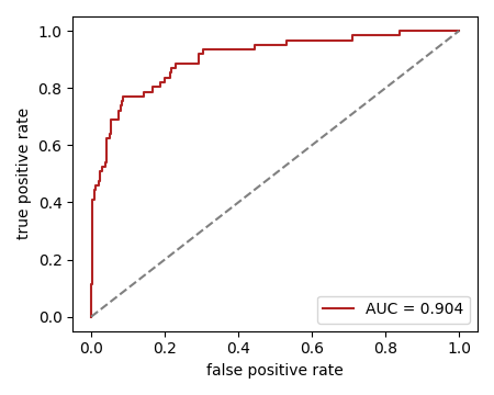
Figure 8.17: ROC curve in python
8.1.9.3 metrics for unsupervised learning
Evaluating a clustering is harder, because in general there is no truth to compare with. The metrics split into two groups: the external ones, which require a known partition and are therefore used mainly on benchmark data or to compare two clusterings with each other, and the internal ones, which judge the geometry of the result alone and are the only ones available in a real application.
Contingency Matrix:
The analogue of the confusion matrix for clustering: it crosses the found clusters with the true groups. It cannot be read directly as a confusion matrix, because the labels of the clusters are arbitrary, and all the external indices below are functions of this table built to be invariant to any renaming.
rand and adjusted rand index:
The Rand index looks at all the pairs of observations and counts the share on which the two partitions agree, that is the pairs placed together in both or separated in both:
\[\begin{equation} RI=\frac{a+b}{\binom{n}{2}} \tag{8.23} \end{equation}\]
where \(a\) is the number of pairs joined in both partitions and \(b\) the number separated in both. Its defect is that it does not go to zero for a random partition. The adjusted Rand index corrects it for chance:
\[\begin{equation} ARI=\frac{RI-E[RI]}{\max(RI)-E[RI]} \tag{8.24} \end{equation}\]
and it is the one to use: it equals one for a perfect match and about zero for an arbitrary grouping.
mutuel information:
Borrowed from information theory, it measures how much knowing the cluster reduces the uncertainty about the true group:
\[\begin{equation} MI(U,V)=\sum_{i}\sum_{j}\frac{\lvert u_i\cap v_j\rvert}{n}\ln\frac{n\lvert u_i\cap v_j\rvert}{\lvert u_i\rvert\lvert v_j\rvert} \tag{8.25} \end{equation}\]
Like the Rand index it exists in a normalized and an adjusted version, and for the same reason.
homogeneity score:
A clustering is homogeneous if every cluster contains observations of a single true group. It is a purity criterion, and it can be made perfect trivially by putting every observation in its own cluster.
completeness score:
The symmetric requirement: all the observations of a given true group are placed in the same cluster. It too can be made perfect trivially, by putting everything into a single cluster. Each of the two scores is therefore useless alone.
V measures:
Their harmonic mean, which is to homogeneity and completeness what the \(F_1\) is to precision and recall. Because the two trivial solutions above fail on the other criterion, the \(V\) measure resists both.
fowlkes-mallows scores:
\[\begin{equation} FM=\sqrt{\frac{TP}{TP+FP}\times\frac{TP}{TP+FN}} \tag{8.26} \end{equation}\]
the geometric mean of a precision and a recall computed on the pairs of observations rather than on the observations themselves.
We now come to the internal indices, the ones that work without any truth.
Silhouette Coefficient:
For each observation \(i\), let \(a(i)\) be its average distance to the other members of its own cluster and \(b(i)\) its average distance to the members of the nearest other cluster. The silhouette is:
\[\begin{equation} s(i)=\frac{b(i)-a(i)}{\max\big(a(i),b(i)\big)} \tag{8.27} \end{equation}\]
It lies between \(-1\) and \(1\). A value close to one means the observation is much closer to its own cluster than to any other, a value near zero that it sits on a border, and a negative value that it would be better placed elsewhere. Its great merit is that it is defined observation by observation, so it can be plotted and not only averaged.
Calinski-Harabasz Index:
\[\begin{equation} CH=\frac{tr(B_k)}{tr(W_k)}\times\frac{n-k}{k-1} \tag{8.28} \end{equation}\]
the ratio of the between cluster dispersion to the within cluster dispersion, corrected for the number of clusters \(k\). It is to be maximized, and it is very fast to compute since it only involves the centres.
Davies-Bouldin Index:
\[\begin{equation} DB=\frac{1}{k}\sum_{i=1}^{k}\max_{j\neq i}\left(\frac{\sigma_i+\sigma_j}{d(c_i,c_j)}\right) \tag{8.29} \end{equation}\]
For each cluster it finds its worst neighbour, the one with which the ratio of the sum of the dispersions to the distance between the centres is largest, and averages these worst cases. Contrary to the two previous indices it is to be minimized.
The natural use of these three indices is to choose the number of clusters, which no algorithm can decide by itself.
In R:
suppressPackageStartupMessages(library(cluster))

set.seed(123)
cl3 <- rbind(
  data.frame(x1 = rnorm(80, 2, .7), x2 = rnorm(80, 2, .7)),
  data.frame(x1 = rnorm(80, 6, .7), x2 = rnorm(80, 3, .7)),
  data.frame(x1 = rnorm(80, 4, .7), x2 = rnorm(80, 6.5, .7)))
D <- dist(cl3)

ch_index <- function(d, cl) {
  k <- length(unique(cl)); n <- nrow(d)
  g <- colMeans(d)
  W <- sum(sapply(split(seq_len(n), cl), function(i)
        sum(sweep(d[i, , drop = FALSE], 2, colMeans(d[i, , drop = FALSE]))^2)))
  B <- sum(sapply(split(seq_len(n), cl), function(i)
        length(i) * sum((colMeans(d[i, , drop = FALSE]) - g)^2)))
  (B / (k - 1)) / (W / (n - k))
}

ks <- 2:8
idx <- do.call(rbind, lapply(ks, function(k) {
  km <- kmeans(cl3, centers = k, nstart = 20)
  data.frame(k = k,
             silhouette = mean(silhouette(km$cluster, D)[, 3]),
             CH = ch_index(cl3, km$cluster),
             within_ss = km$tot.withinss)
}))

i1 <- ggplot(idx, aes(k, silhouette)) + geom_line() + geom_point() +
  geom_vline(xintercept = idx$k[which.max(idx$silhouette)], linetype = 2, colour = "firebrick") +
  labs(title = "silhouette (maximize)") + theme_minimal()
i2 <- ggplot(idx, aes(k, CH)) + geom_line() + geom_point() +
  geom_vline(xintercept = idx$k[which.max(idx$CH)], linetype = 2, colour = "firebrick") +
  labs(title = "Calinski-Harabasz (maximize)") + theme_minimal()
i3 <- ggplot(idx, aes(k, within_ss)) + geom_line() + geom_point() +
  labs(title = "within sum of squares (elbow)") + theme_minimal()

i1 + i2 + i3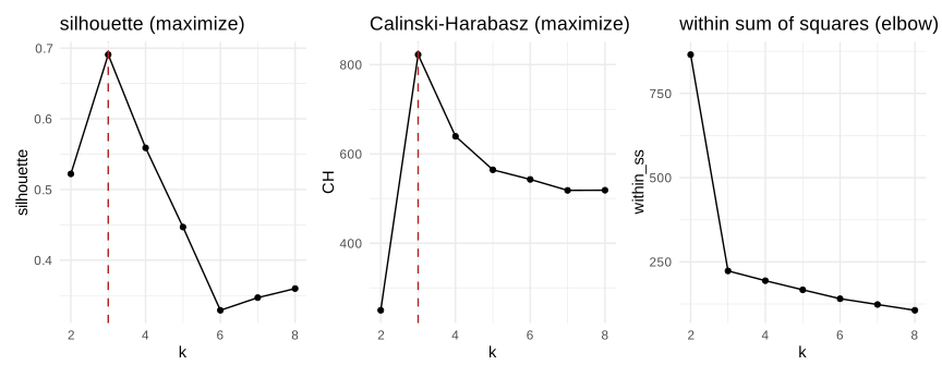
Figure 8.18: choosing the number of clusters with three internal indices
The first two indices peak at the number of groups we simulated, and the third shows the familiar elbow at the same place. The elbow is the oldest of the three and the least reliable, because reading the position of a bend is subjective, whereas a maximum is not.
The silhouette can also be displayed observation by observation, which says much more than its average.
par(mfrow = c(1, 2))
km3 <- kmeans(cl3, centers = 3, nstart = 20)
km6 <- kmeans(cl3, centers = 6, nstart = 20)
plot(silhouette(km3$cluster, D), main = "k = 3", col = "grey40", border = NA)
plot(silhouette(km6$cluster, D), main = "k = 6", col = "grey40", border = NA)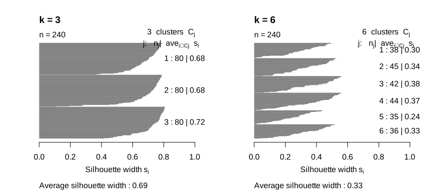
Figure 8.19: silhouette plot for a good and a bad number of clusters
With three clusters the bars are long and almost all positive. With six, several bars are short and some become negative, which signals observations that have been placed in a cluster they do not belong to: the partition has been cut too finely.
In Python:
from sklearn.cluster import KMeans
from sklearn.metrics import (silhouette_score, calinski_harabasz_score,
                             davies_bouldin_score, adjusted_rand_score,
                             v_measure_score)

X = np.asarray(cl3_py, dtype=float)
truth = np.repeat([0, 1, 2], 80)

rows = []
for k in range(2, 9):
    lab = KMeans(n_clusters=k, n_init=20, random_state=0).fit_predict(X)
    rows.append({"k": k,
                 "silhouette": round(silhouette_score(X, lab), 4),
                 "CH": round(calinski_harabasz_score(X, lab), 1),
                 "DB": round(davies_bouldin_score(X, lab), 4),
                 "ARI_vs_truth": round(adjusted_rand_score(truth, lab), 4),
                 "V_measure": round(v_measure_score(truth, lab), 4)})

clust_py = pd.DataFrame(rows)| k | silhouette | CH | DB | ARI_vs_truth | V_measure |
|---|---|---|---|---|---|
| 2 | 0.5221 | 249.7 | 0.7122 | 0.5694 | 0.7337 |
| 3 | 0.6908 | 822.3 | 0.4236 | 1.0000 | 1.0000 |
| 4 | 0.5589 | 639.4 | 0.7613 | 0.8687 | 0.9050 |
| 5 | 0.4394 | 564.5 | 0.9727 | 0.7160 | 0.8115 |
| 6 | 0.3292 | 542.8 | 1.1509 | 0.5709 | 0.7614 |
| 7 | 0.3421 | 517.3 | 1.0350 | 0.5172 | 0.7283 |
| 8 | 0.3592 | 518.6 | 0.9419 | 0.4600 | 0.6976 |
The table gathers the two families side by side. The silhouette and the Calinski-Harabasz index reach their maximum, and the Davies-Bouldin index its minimum, at the same value of \(k\), and the two external indices, which are allowed to look at the truth, confirm that this value is indeed the right one. In a real application only the first three columns would be available, and this is precisely why they were designed.