5.3 Non normality
In the DGP model, we have two parts, the deterministic part, represented by the regressors, and the stochastic one, by the theoretical variable \(\varepsilon\). For the OLS estimator to be consistent (or unbiased), we do not need this assumption. However, the related statistic tests such as t-test and F-test used to assess the estimated model have been derived from that assumption. Therefore, the model will be less accurate for inferences but not for prediction since for the latter purpose, there exist other types of assessment such as the hold out samples as in machine learning.
Models fitted with large samples are not much concerned by the normality since they use the central limit theorem (see ??) that approximates, significantly, the results. Unless we know the exact distribution (such as Poisson, Gamma, etc.), we should use the Generalized linear models GLM (discussed in the following chapters). Even with small samples, Green said that this assumption could be discarded in most practical cases (Green 2018).
5.3.1 Testing the normality assumption
Since the theoretical error term \(\varepsilon\) is never known, the residuals resulting from the estimated model will be used instead to test this assumption. There exist several tests to test this assumption. In this subsection, We introduce the most popular ones.
5.3.1.1 Visual Methods
The histogram :
The histogram is the frequency distribution of some variable. It is the most popular plot used to visualize frequency distributions. Therefore, if the distribution of the variable under study is normal, then we expect its histogram to be close to the well-known bell shape of the normal distribution. The picture below has two plots, the left one is drawn from the normal distribution and the right one from the Beta distribution. As you can see, it is clear to recognize that the lower one is not normally distributed.
suppressPackageStartupMessages(library(patchwork))

set.seed(1)
x1 <- rnorm(1000, 5, 10)
x2 <- rbeta(1000, 5, 0.5)
df <- tibble(x1=x1, x2=x2)
g1 <- ggplot(df, aes(x1))+
  geom_histogram( aes(y=..density..), fill='lightblue', bins = 50)+
  stat_function(fun = dnorm,
                args = list(mean = mean(df$x1), sd = sd(df$x1)))
g2 <- ggplot(df, aes(x2))+
  geom_histogram(aes(y=..density..), fill='lightblue', bins = 50)+
   stat_function(fun = dnorm,
                args = list(mean = mean(df$x2), sd = sd(df$x2)))

g1+g2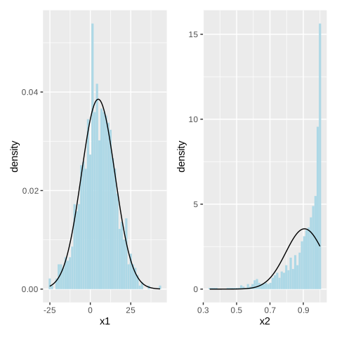
Figure 5.8: Check normality with histogram in R
In Python
import numpy as np
import pandas as pd
import matplotlib.pyplot as plt
import matplotlib
np.random.seed(1)
x1 = np.random.normal(5,10,1000)
x2 = np.random.beta(5, 0.5, 1000)
y2 = np.random.normal(np.mean(x2), np.std(x2), 1000)
df = pd.DataFrame({'x1':x1, 'x2':x2, 'y2':y2})

matplotlib.style.use('classic')

fig= plt.figure(figsize=(5,5))
plt.subplot(211)
df.x1.hist(bins=50,density=True, grid=False)
df.x1.plot.kde(color='red')
plt.subplot(212)
df.x2.hist(bins=50, density=True, grid=False)
df.y2.plot.kde(color='red')
plt.savefig('histplot.png')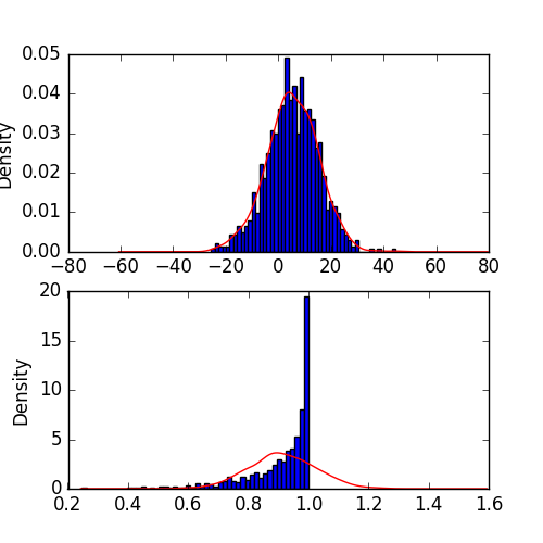
Figure 5.9: Check normality with histogram in Python
The stem-and-leaf plot:
The idea behind this plot is simple. We take the values of the variable of interest, regardless whether it is discrete or continuous, then we separate the last digit from the first ones for each value. The first part is called stem, and the last one is called leaf. This plot is a diagram rather than a graph, and to understand how made, suppose that we have some data drawn from the Poisson distribution as follows (using R).
[out] [1] 3 4 4 5 8 9 16 16 17 19 21 23 26 27 32 32 33 34 39 40Then the plot will be:
[out]
[out]   The decimal point is 1 digit(s) to the right of the |
[out]
[out]   0 | 344589
[out]   1 | 6679
[out]   2 | 1367
[out]   3 | 22349
[out]   4 | 0
In Python we should install a package called stemgraphic as follows:
import numpy as np
import stemgraphic
rng=np.random.RandomState(seed=1)
x=list(rng.poisson(lam=5, size=5))+list(rng.poisson(lam=15, size=5))+list(rng.poisson(lam=25, size=5))+list(rng.poisson(lam=35, size=5))
stemgraphic.stem_graphic(x, scale=10)
plt.show()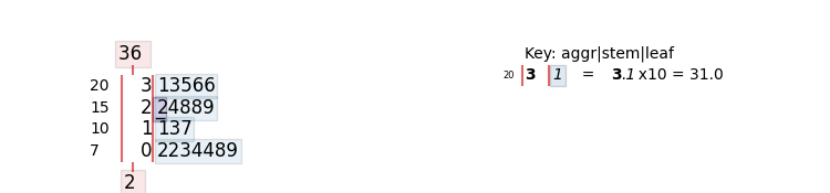
Figure 5.10: stem-and-leaf plot in Python
Unlike R, we have an extra column in the left shows how many instances in each line.
The boxplot:
The boxplot is a graphical representation of the popular five statistics, maximum, minimum, the first quartile, the third quartile, and the median. It is more useful to represent categorical variables, but it can also be used for continuous ones. The code of the plot below in this gist.
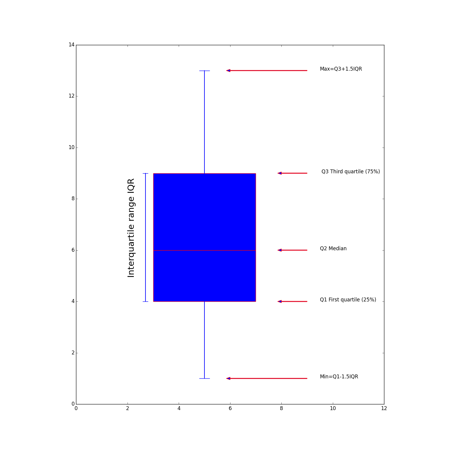
Figure 5.11: Box plot
Let us create two box plots for two different distributions. The first one is for the normal distribution and the second one for the beta distribution.
set.seed(1)
x_normal <- rnorm(n=200, mean=8, sd=3)
x_beta <- rbeta(n=200, shape1 = 3, shape2 = 0.5)
x <- 1:200


df <- tibble(x=x, x_normal=x_normal, x_beta=x_beta)
g1 <- ggplot(df, aes(x, x_normal))+
  geom_boxplot( fill='lightblue')
g2 <- ggplot(df, aes(x, x_beta))+
  geom_boxplot( fill='lightblue')

g1+g2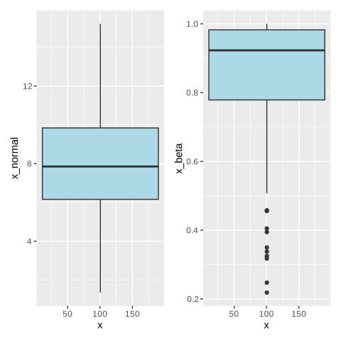
Figure 5.12: Box plot in R
Any data that has a boxplot, with a shape similar to the right one in the above figure, is normally distributed. As such, the second box plot could not characterize a normal distribution.
import numpy as np
import matplotlib.pyplot as plt
import pandas as pd
fig, ax = plt.subplots(1, 2)
rng=np.random.RandomState(seed=1)
x_normal=rng.normal(loc=8, scale=3, size=200)
x_beta=rng.beta(a=3, b=0.5, size=200)
dff=pd.DataFrame({"x_normal": x_normal, "x_beta":x_beta})
plt.clf()
plt.close()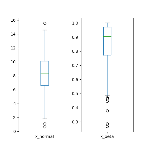
Figure 5.13: Box plot in Python
The P-P plot:
This one plots the probability distribution of the data at hand against any other theoretical distribution (in our case, the normal distribution). If the points lie around the line of 45° (\(y=x\)), we can thus conclude that the two distributions are closer two each other. Hence, the distribution of our data can be approximated by that distribution.
In R we will use the package qqplotr. Again, we will use the previous data stored in df.
suppressPackageStartupMessages(library(qqplotr))
g1 <- ggplot(df, aes(sample=x_normal)) +
    stat_pp_band() +
    stat_pp_line() +
    stat_pp_point() +
    labs(x = "Normal distribution", y = "Data distribution")
g2 <- ggplot(df, aes(sample=x_beta)) +
    stat_pp_band() +
    stat_pp_line() +
    stat_pp_point() +
    labs(x = "Beta distribution", y = "Data distribution")
g1+g2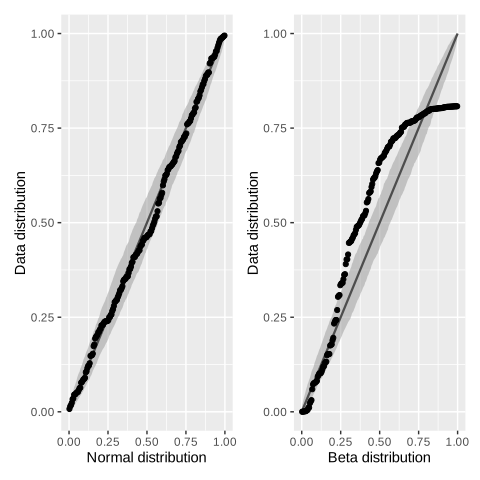
Figure 5.14: p-p plot in R
As we can see, the most observations in the right plot are outside the confidence intervals, which means that the data is not normally distributed.
It should be noted that the function stat_pp_band can use many other distributions. For instance we can check whether the x_beta follows the beta distribution or not as follows:
d <- "beta"
param <- list(shape1=3, shape2=0.5)
de <- TRUE
g <- ggplot(df, aes(sample=x_beta)) +
    stat_pp_band(distribution = d, dparams = param) +
    stat_pp_line(distribution = d, dparams = param) +
    stat_pp_point(distribution = d, dparams = param) +
    labs(x = "Beta distribution", y = "Data distribution")
g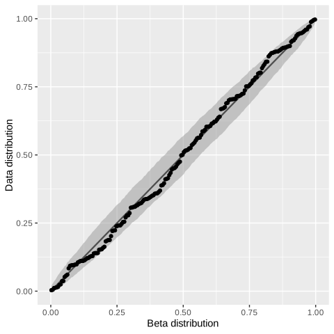
Figure 5.15: p-p plot for Beta dist in R
As we see, the distribution of the x_beta matches that of Beta.
In Python:
To visualize, both p-p plot ans q-q plot, will use statsmodels package.
import statsmodels.api as sm
fig, ax = plt.subplots(1, 2)
plot_norm = sm.ProbPlot(dff.x_normal.values, fit=True)
plot_norm.ppplot(ax=ax[0], line="45")
plot_beta = sm.ProbPlot(dff.x_beta.values, fit=True)
plot_beta.ppplot(ax=ax[1], line="45")
plt.show()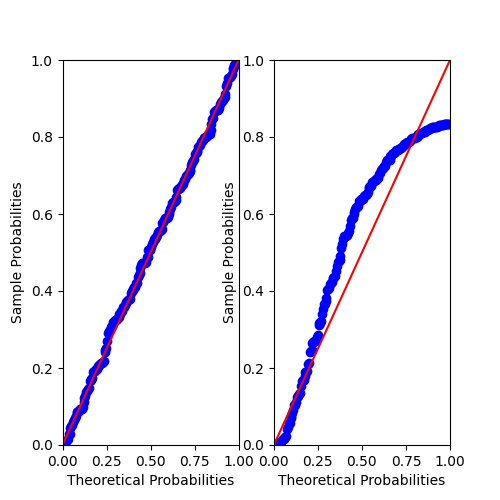
Figure 5.16: p-p plot in Python
The Q-Q plot:
Unlike the previous one, this one plots the quantiles (not the probabilities) of both distributions against each other. Also, the intercept and the slope of the line around which the points should lie are the mean and the standard deviation of the date respectively.
g1 <- ggplot(df, aes(sample=x_normal)) +
    stat_qq_band() +
    stat_qq_line() +
    stat_qq_point() +
    labs(x = "Normal quatile", y = "Data quantile")
g2 <- ggplot(df, aes(sample=x_beta)) +
    stat_qq_band() +
    stat_qq_line() +
    stat_qq_point() +
    labs(x = "Beta quantile", y = "Data quantile")
g1+g2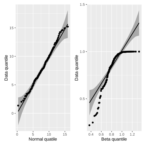
Figure 5.17: q-q plot in R
Again, the second plot shows that the data is not normally distributed.
Note: As we did previously, we can also check the beta distribution bu specifying the distribution argument in the stat_qq_band function.
g <- ggplot(df, aes(sample=x_beta)) +
    stat_qq_band(distribution = "beta", dparams = list(3, 0.5)) +
    stat_qq_line() +
    stat_qq_point() +
    labs(x = "Beta quantile", y = "Data quantile")
g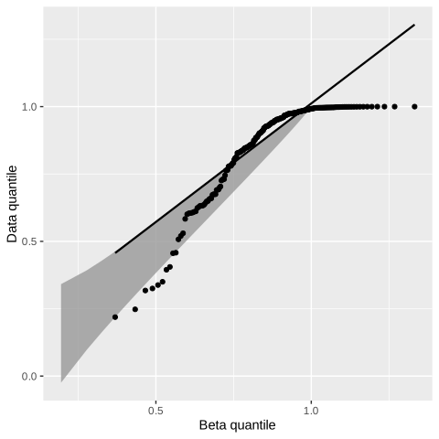
Figure 5.18: q-q plot in R
In python we will call the statsmodels package.
import statsmodels.api as sm
fig, ax = plt.subplots(1, 2)
plot_norm = sm.ProbPlot(dff.x_normal.values)
plot_norm.qqplot(ax=ax[0], line="s")
plot_beta = sm.ProbPlot(dff.x_beta.values)
plot_beta.qqplot(ax=ax[1], line="s")
plt.show()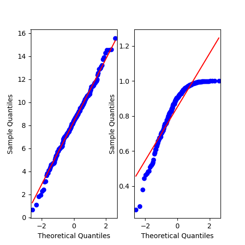
Figure 5.19: q-q plot in Python
5.3.1.2 Kolmogorov-Smirnov test KS
Invented by Andrey Kolmogorov and Nikolai Smirnov. This test is used to compare the observed frequency distribution with any reference probability distribution (the normal distribution to test normality assumption). The idea behind this test is to check the distance that separates the observed distribution \(\widehat F(x)\) given by:
\[\begin{equation} \widehat F(x)=\frac{1}{n}\sum\limits_{i}^{n}1(x_i\leqslant x) \end{equation}\]
Where \(1(x_i\leqslant x)\) is the indicator function.
From that that we are testing for \(F(x)\):
\[\begin{equation} D=\underset{x}{sup}\bigg|\widehat F(x)-F(x)\bigg| \tag{5.58} \end{equation}\]
where \(\underset{x}{sup}\) is the supermum of the set of distances. The value of this statistic should be compared to the critical values provided by Smirnov. If the computed value is higher than the critical one, we should reject the null hypothesis hence the normality assumption.
The distribution of the random variable \(D\) is based on the following distribution known as Kolmogorov distribution:
\[\begin{equation} K(x)=1-2\sum\limits_{k=1}^{\infty}(-1)^{k-1}exp\bigg(-2k^2x^2\bigg) \end{equation}\]
Such that \(\sqrt{n}D\xrightarrow{n\rightarrow\infty}K(x)\)
It should be noted that those critical values required the reference distribution to be fully determined. That is, the mean and the standard deviation should be defined a priori. If not, however, and we do not have but estimate them from the sample, then we should use the critical values provided by another version of this test called Lilliefors test instead,
5.3.1.3 Lilliefors corrected test
named after Hubert Lilliefors, This test is based on the KS test, but provides the suitable critical values when the parameters of the normal distribution are estimated from the sample.
5.3.1.4 Shapiro-Wilk test
This test is defined as follows:
\[\begin{equation} W=\frac{\bigg(\sum\limits_{i=1}^n a_ix_{(i)}\bigg)^2}{\sum\limits_{i=1}^n\big(x_i-\bar x\big)^2} \tag{5.59} \end{equation}\]
where \(x_{(i)}\) is the \(i^{th}\) smallest number in the sample (called also the \(i^{th}\) order statistic), and the coefficients are \(a_i\) are computed from:
\[\begin{equation} (a_1,..,a_n)=\frac{m^tV^{-1}}{\sqrt{m^tV^{-1}V^{-1}m}} \end{equation}\]
Where \(m\) is the vector of the expected values of the order statistics sampled from the standard normal distribution, and \(V\) is the corresponding covariance matrix.
The values of this test is always less than one. So values closer to one are in favor of the normality assumption.
5.3.1.5 Anderson-Darling test
The advantage of this test over the previous ones, is that it does not require the parameters of the reference distribution being tested. Unlike KS test that uses the absolute distance, this one uses the quadratic distance instead as follows:
\[\begin{equation} A^2=n\int\limits_{-\infty}^{\infty}\frac{\bigg(\widehat F(x)-F(x)\bigg)^2}{F(x)\bigg(1-F(x)\bigg)}dF(x) \end{equation}\]
Which can be simplified by:
\[\begin{equation} A^2=-n-\sum\limits_{i=1}^{n}\frac{2i-1}{n}[lnF(x_i)+ln\big(1-F(x_{n+1-i})\big)] \tag{5.60} \end{equation}\]
5.3.1.6 Cramer-von Mises test
This test is like the previous one without the numerator:
\[\begin{equation} W^2=n\int\limits_{-\infty}^{\infty}\bigg(\widehat F(x)-F(x)\bigg)^2dF(x) \end{equation}\]
And simplified by:
\[\begin{equation} W^2=\frac{1}{12n}+\sum\limits_{i=1}^{n}\Bigg[\frac{2i-1}{2n}-F(x_i)\Bigg]^2 \tag{5.61} \end{equation}\]
Values larger than the tabulated ones leas to reject the distribution being tested.
5.3.1.7 Jarque-Bera test JB
Introduced fist by Carlos Jarque and Anil K. Bera. This test check if the skewness (\(S=\frac{\mu_3}{\sigma^3}\)) and the kurtosis (\(K=\frac{\mu_4}{\sigma^4}\)) matches those of the normal distribution. That is, the data that has \(S\) close to zero and \(K\) close to 3 is likely to come from the normal distribution. JB test is a combination of those two measures by the following:
\[\begin{equation} JB=\frac{n}{6}\bigg(s^2+\frac{1}{4}(K-3)^2\bigg) \tag{5.62} \end{equation}\]
When the sample skewness \(S=\frac{\widehat\mu_3}{\widehat\sigma^3}\) and the sample kurtosis are used, this test follows the chi-squared distribution with two degrees of freedom.
In R:
Again, we will use the data stored in df to apply the above tests.
Kolmogorov-Smirnov test KS:
[out]
[out]   Asymptotic one-sample Kolmogorov-Smirnov test
[out]
[out] data:  df$x_normal
[out] D = 0.052201, p-value = 0.647
[out] alternative hypothesis: two-sided
Since the p-value is greater than the popular threshold \(0.05\), we cannot reject the null hypothesis that the data is normally distributed.
[out]
[out]   Asymptotic one-sample Kolmogorov-Smirnov test
[out]
[out] data:  df$x_beta
[out] D = 0.19297, p-value = 6.8e-07
[out] alternative hypothesis: two-sided
Unlike the data sampled from the beta distribution, its p-value \(7.8e-07\) is very tiny suggesting the rejection of the null hypothesis of normality
This function can also be used to check if two variables come from the same distribution.
[out]
[out]   Asymptotic two-sample Kolmogorov-Smirnov test
[out]
[out] data:  df$x_normal and df$x_beta
[out] D = 1, p-value < 2.2e-16
[out] alternative hypothesis: two-sided
Shapiro-Wilk test:
[out]
[out]   Shapiro-Wilk normality test
[out]
[out] data:  df$x_normal
[out] W = 0.99274, p-value = 0.4272[out]
[out] Shapiro-Wilk normality test
[out]
[out] data: df$x_beta
[out] W = 0.81384, p-value = 1.019e-14Jarque-Bera test JB:
This test can be applied through the normtest package as follows.
[out]
[out]   Jarque-Bera test for normality
[out]
[out] data:  df$x_normal
[out] JB = 1.671, p-value = 0.402[out]
[out] Jarque-Bera test for normality
[out]
[out] data: df$x_beta
[out] JB = 100.51, p-value < 2.2e-16Lilliefors corrected test:
For this test and the following ones, we use the nortest package.
[out]
[out]   Lilliefors (Kolmogorov-Smirnov) normality test
[out]
[out] data:  df$x_normal
[out] D = 0.052201, p-value = 0.203[out]
[out] Lilliefors (Kolmogorov-Smirnov) normality test
[out]
[out] data: df$x_beta
[out] D = 0.19297, p-value < 2.2e-16Anderson-Darling test:
[out]
[out]   Anderson-Darling normality test
[out]
[out] data:  df$x_normal
[out] A = 0.33781, p-value = 0.5025[out]
[out] Anderson-Darling normality test
[out]
[out] data: df$x_beta
[out] A = 11.793, p-value < 2.2e-16Cramer-von Mises test:
[out]
[out]   Cramer-von Mises normality test
[out]
[out] data:  df$x_normal
[out] W = 0.055915, p-value = 0.4265[out]
[out] Cramer-von Mises normality test
[out]
[out] data: df$x_beta
[out] W = 2.0392, p-value = 7.37e-10Kolmogorov-Smirnov test KS:
In python, we use the scipy package to perform this test.
[out] KstestResult(statistic=0.09232544866435122, pvalue=0.06198680490844932, statistic_location=6.943250460519444, statistic_sign=-1)[out] KstestResult(statistic=0.658658763145334, pvalue=1.2136564931435564e-85, statistic_location=0.46395152846928106, statistic_sign=-1)To test if the two data come from the same distribution, we execute the following script.
[out] KstestResult(statistic=0.995, pvalue=7.770573798088942e-117, statistic_location=0.9999783433977696, statistic_sign=-1)Since the p-value is very tiny, we conclude that the two data have different distributions.
Shapiro-Wilk test:
[out] ShapiroResult(statistic=0.9958661900981383, pvalue=0.8669629256600266)[out] ShapiroResult(statistic=0.8475490543331776, pvalue=3.275253917460355e-13)Jarque-Bera test JB:
[out] SignificanceResult(statistic=0.3099628619177972, pvalue=0.8564310804398949)[out] SignificanceResult(statistic=84.52601732558254, pvalue=4.419860365592142e-19)Lilliefors corrected test:
For this test we will use the statsmodelspackage
[out] (0.037467941269319904, 0.7162544216034896)[out] (0.16621524671074217, 0.0009999999999998899)Anderson-Darling test:
Again, we will use the scipy package.
[out] AndersonResult(statistic=0.20105337327842676, critical_values=array([0.565, 0.644, 0.772, 0.901, 1.071]), significance_level=array([15. , 10. ,  5. ,  2.5,  1. ]), fit_result=  params: FitParams(loc=8.320066444543846, scale=2.7369889959520455)
[out]  success: True
[out]  message: '`anderson` successfully fit the distribution to the data.')
If the threshold of \(0.05\) is chosen, then the critical value is \(0.772\).
Cramer-von Mises test:
[out] CramerVonMisesResult(statistic=0.38630093938822835, pvalue=0.07845933337170297)[out] CramerVonMisesResult(statistic=30.43430874827928, pvalue=7.580966743248041e-09)5.3.2 Bootstrapped confidence intervals
If the normality assumption is not satisfied, we will not be able to apply the popular statistics t-test and F-test to test the significance of the outputs via the confidence intervals or their standard errors.
The bootstrapping method is an alternative way to build confidence intervals regardless of the normality assumption. The idea behind this method is repeatedly sampling with replacement from the data at hand. Then for each sample, we compute the output we want. Finally, we use the distribution of all the resulting values for that output to get the confidence intervals.
This method gained popularity in recent decades due to the increasing power of computers that allows the use of simulation techniques with less amount of time. For mor depth see(MacKinnon 2002).
In R:
First we will simulate some data to work with
set.seed(12)
epsilon <- rnorm(70)
x <- rnorm(n=70, mean=15, sd=3)
y <- 1.2+2.5*x+epsilon
df_boot <- data.frame(y=y, x=x)
The confidence intervals computed from the usual t-test are the following.
[out]                 2.5 %   97.5 %
[out] (Intercept) 0.4385654 3.059716
[out] x           2.3781854 2.549401
Now let us use the bootstrap method to compute the confidence intervals.
Before starting coding, we have to understand how this technique is performed in the regression model using the simple linear regression model.
First, we fit a model with the original data, then take out the fitted values and the residuals as follows:
Then, with 1000 rounds so that at each round, we shuffle the resids set (that stores the residuals) and add them to the fitted_values set to get new values for the response variable \(y\). Next, we regress the resulted response variable to the explanatory variable to get a new slope and a new intercept.
In R, the bootstrap method is provided from the boot package. The function boot required the data used to sample from (as its first parameter), which is here the resids set, and a function to compute the outputs that we want, then the number of replications (rounds)
coef_boot <- function(resids, index){
  y <- fitted_values+resids[index]
  model <- lm(y~x)
  coef(model)
}
To get the slope, we set the argument \(index=2\) (1 for the intercept)
library(boot)
boot_model <- boot(resids, coef_boot, R=1000)
# it uses 95% confidence by default
boot.ci(boot_model, index=2)
[out] BOOTSTRAP CONFIDENCE INTERVAL CALCULATIONS
[out] Based on 1000 bootstrap replicates
[out]
[out] CALL :
[out] boot.ci(boot.out = boot_model, index = 2)
[out]
[out] Intervals :
[out] Level Normal Basic
[out] 95% ( 2.378, 2.548 ) ( 2.380, 2.550 )
[out]
[out] Level Percentile BCa
[out] 95% ( 2.377, 2.548 ) ( 2.377, 2.547 )
[out] Calculations and Intervals on Original ScaleAs we see, There exist for types of intervals. The most used one is the bias-corrected accelerated interval (BCa)(Davison.C and Hinkley.D 1997) that corrects the bias and the skeweness of the distribution.
Let us first remove the data from R to Python.
Now we fit the model, and take out the fitted values and the residuals
import statsmodels.formula.api as smf
model = smf.ols("y~x", data=df_boot_py).fit()
fitted_values = model.fittedvalues
resids = model.resid
Then we run the bootstrapping method.
import pandas as pd
import numpy as np

# create an empty list
bootstrap=[]

# run 1000 replications
for i in np.arange(1000):
  # at each iteration set the seed to let the example reproducible
  np.random.seed(i)
  # sample from the original residuals
  index=np.random.choice(len(resids), size=len(resids))
  # generate the response from the randomized data
  y=fitted_values+resids[index]
  x = df_boot_py.x
  data=pd.DataFrame({"y":y, "x":x})
  # fit the linear model
  model = smf.ols("y~x", data=data ).fit()
  # store the slop in the bootstrap list, for the intercept we use 0 instead
  bootstrap.append(model.params[1])

# compute the confidence intervals
(np.quantile(bootstrap, 0.025), np.quantile(bootstrap, 0.975))
[out] (2.3761388647957165, 2.545995025676658)