3.8 Selection of regressors
At least in economic fields, variables are often influenced by more than one regressor, which justifies the use of the multiple linear models. However, unlike the simple linear model, many questions arise in this case, such as, How can we define these regressors, how affect adding or deleting some regressors the dependent variable, what is the effect of omitting relevant variables or including irrelevant variables, etc.
In practice, the variable that may influence the dependent variable can be suggested either by the underlying theory or by the investigator based on his experience. However, sometimes it is too hard to determine exactly the right regressors, that is why econometric models are used to help the investigator to maintain the relevant variables and exclude the irrelevant ones.
As said before, the OLS estimators are unbiased, provided that the regressors in the estimated model are the same as in the DGP model. What happens then if some of these regressors omitted from the estimated model (relevant variables) or other new regressors are included (irrelevant variables).
In general, we have three cases:
1- The estimated model has the same set of regressors as in the DGP model. We have treated this case earlier, and it remains to show how computing only a subset of the OLS estimators if we are interested in only the associated regressors.
2- The estimated model omits a subset of the DGP regressors.
3- In addition to the DGP regressors, the estimated model includes new ones that are not in the DGP model.
3.8.1 Including all the DGP regressors
Suppose that the matrix \(X\) in the true model \(y=X\beta+\varepsilon\) is split into two groups \(X=[X_IX_{II}]\), \(X_I\) is \(n\times (k-\mathrm g)\) and contains the constant term, and \(X_{II}\) is \(n\times \mathrm g\). Notice that \(X_I\) has \(k-\mathrm g-1\) variables, and \(X_{II}\) has exactly \(\mathrm g\) variables.
This reformulation implies that the vector \(\beta\) will be also partitioned into two vectors superposed together:
\[\begin{equation*} \beta= \begin{pmatrix} \beta_I\\ \beta_{II} \end{pmatrix} \end{equation*}\]
Where \(\beta_I\) has \(k-\mathrm g\) elements, and \(\beta_{II}\) has \(\mathrm g\) elements.
Using these partitions, the true model will be rewritten as:
\[\begin{equation} y=[X_IX_{II}] \begin{pmatrix}\beta_I\\ \beta_{II} \end{pmatrix} +\varepsilon=X_I\beta_I+X_{II}\beta_{II}+\varepsilon \tag{3.44} \end{equation}\]
And the estimated model with all the DGP regressors included, from now on called the unrestricted model, is:
\[\begin{equation} y=X_I\widehat\beta_I+X_{II}\widehat\beta_{II}+e \tag{3.45} \end{equation}\]
While the OLS estimators vector will be:
\[\begin{align*} \widehat\beta=\big(X^tX\big)^{-1}X^ty\implies \begin{pmatrix}\widehat\beta_I\\\widehat\beta_{II}\end{pmatrix}&=\bigg[\begin{pmatrix}X^t_I\\X^t_{II}\end{pmatrix}(X_IX_{II})\bigg]^{-1}\begin{pmatrix}X^t_I\\X^t_{II}\end{pmatrix}y\\ &=\begin{pmatrix}X^t_IX_I&X^t_IX_{II}\\X^t_{II}X_I&X^t_{II}X_{II}\end{pmatrix}^{-1}\begin{pmatrix}X^t_Iy\\X^t_{II}y\end{pmatrix} \end{align*}\]
Definition 3.7 Let \(A=\begin{pmatrix}A_{11}&A_{12}\\A_{21}&A_{22}\end{pmatrix}\) be a \(2\times 2\) block matrix where \(A_{11}\) and \(A_{22}\) are non singular square matrices, so the inverse of this matrix can be rewritten in two different ways:
\[\begin{equation*} A^{-1}= \begin{bmatrix} B_{11}&-B_{11}A_{12}A_{22}^{-1}\\ -A_{22}^{-1}A_{21}B_{11}&A_{22}^{-1}+A_{22}^{-1}A_{21}B_{11}A_{12}A_{22}^{-1} \end{bmatrix} \end{equation*}\]
Where \(B_{11}=\big(A_{11}-A_{12}A_{22}^{-1}A_{21}\big)^{-1}\)
This formula is preferred if we are interested in the first line of this matrix.
\[\begin{equation*} A^{-1}= \begin{bmatrix} A_{11}^{-1}+A_{11}^{-1}A_{12}B_{22}A_{21}A_{11}^{-1}&-A_{11}^{-1}A_{12}B_{22}\\ -B_{22}A_{21}A_{11}^{-1}&B_{22} \end{bmatrix} \end{equation*}\]
Where \(B_{22}=\big(A_{22}-A_{21}A_{11}^{-1}A_{12}\big)^{-1}\)
This formula is preferred if we are interested in the second line.
For the proof see(Whitelaw 1991).
According to 3.7, the blocks of the above matrix are:
- \(A_{11}=X^t_IX_I\).
- \(A_{12}=X^t_IX_{II}\).
- \(A_{21}=X^t_{II}X_I\).
- \(A_{22}=X^t_{II}X_{II}\).
And the main elements of its inverse (\(B_{11}\), \(B_{22}\)) are:
\[\begin{align*} B_{11}&=\bigg(X^t_IX_I-X^t_IX_{II}\big(X^t_{II}X_{II}\big)^{-1}X^t_{II}X_I\bigg)^{-1}\\ &=\bigg(X^t_I\bigg(I-X_{II}\big(X^t_{II}X_{II}\big)^{-1}X^t_{II}\bigg)X_I\bigg)^{-1}\\ &=\bigg(X^t_IM_{II}X_I\bigg)^{-1} \end{align*}\]
\[\begin{align*} B_{22}&=\bigg(X^t_{II}X_{II}-X^t_{II}X_I\big(X^t_IX_I\big)^{-1}X^t_IX_{II}\bigg)^{-1}\\ &=\bigg(X^t_{II}\bigg(I-X_I\big(X^t_IX_I\big)^{-1}X^t_I\bigg)X_{II}\bigg)^{-1}\\ &=\bigg(X^t_{II}M_IX_{II}\bigg)^{-1} \end{align*}\]
Therefore, if the investigator is only interested in the effects of the regressors in the matrix \(X_I\), then the corresponding coefficients in \(\widehat\beta_I\) will be:
\[\begin{align} \widehat\beta_I&=B_{11}X^t_Iy-B_{11}A_{12}A_{22}^{-1}X^t_{II}y\notag\\ &=\big(X^t_IM_{II}X_I\big)^{-1}X^t_Iy-\big(X^t_IM_{II}X_I\big)^{-1}X^t_IX_{II}\big(X^t_{II}X_{II}\big)^{-1}X^t_{II}y\notag\\ &=\big(X^t_IM_{II}X_I\big)^{-1}X^t_I\big(I-X_{II}\big(X^t_{II}X_{II}\big)^{-1}X^t_{II}\big)y\notag\\ \widehat\beta_I&=\big(X^t_IM_{II}X_I\big)^{-1}X^t_IM_{II}y \tag{3.46} \end{align}\]
Notice that the estimates of \(\widehat\beta_I\) using this formula are the same as their corresponding in the original one \(\widehat\beta\), with the only difference that \(\widehat\beta_I\) here, is computed separately.
If instead one is interested in the regressors stored in the matrix \(X_{II}\), then he/she can use the same formula (3.46) after changing the subscripts to the right ones as follows:
\[\begin{equation} \widehat\beta_{II}=\bigg(X^t_{II}M_IX_{II}\bigg)^{-1}X^t_{II}M_Iy \tag{3.47} \end{equation}\]
By the same way, the variance matrix of \(\widehat\beta_I\) can also be computed separately. First, we reformulate (3.46) by substituting y from (3.44):
\[\begin{align*} \widehat\beta_I&=\big(X^t_IM_{II}X_I\big)^{-1}X^t_IM_{II}y\\ &=\big(X^t_IM_{II}X_I\big)^{-1}X^t_IM_{II}\big(X_I\beta_I+X_{II}\beta_{II}+\varepsilon\big)\\ &=\underbrace{\big(X^t_IM_{II}X_I\big)^{-1}X^t_IM_{II}X_I}_{=I}\beta_I+\big(X^t_IM_{II}X_I\big)X^t_I\underbrace{M_{II}X_{II}}_{=0}\beta_{II}+\big(X^t_IM_{II}X_I\big)X^t_IM_{II}\varepsilon \end{align*}\]
The expression \(M_{II}X_{II}=0\) is deduced from \(MX=0\) (see 3.3).
Using the above expression, the variance of \(\widehat\beta_I\) will be:
\[\begin{align*} Var(\widehat\beta_I)&=E\bigg[(\widehat\beta_I-\beta_I)(\widehat\beta_I-\beta_I)^t\bigg]\\ &=\big(X^t_IM_{II}X_I\big)^{-1}X^t_IM_{II}\underbrace{E(\varepsilon\varepsilon^t)}_{=\sigma^2I}M_{II}X_I\big(X^t_IM_{II}X_I\big)^{-1}\\ &=\sigma^2\underbrace{\big(X^t_IM_{II}X_I\big)^{-1}\big(X^t_I\overbrace{M_{II}M_{II}}^{=M_{II}}X_I\big)}_{=I}\big(X^t_IM_{II}X_I\big)^{-1}\\ Var(\widehat\beta_I)&=\sigma^2\big(X^t_IM_{II}X_I\big)^{-1} \end{align*}\]
And hence the estimated variance matrix will be:
\[\begin{equation} Var(\widehat\beta_I)=s^2\big(X^t_IM_{II}X_I\big)^{-1} \tag{3.48} \end{equation}\]
It should be noted that:
\[\begin{equation*} X^te= \begin{pmatrix} X^t_I\\X^t_{II} \end{pmatrix} e= \begin{pmatrix} X^t_Ie\\X^t_{II}e \end{pmatrix} =0\implies \begin{cases} X^t_Ie=0\\X^t_{II}e=0 \end{cases} \end{equation*}\]
There exists an alternative way to extract the formula of \(\widehat\beta_I\) from the unrestricted model:
\[\begin{align*} &\begin{pmatrix} X^t_IX_I&X^t_IX_{II}\\ X^t_{II}X_I&X^t_{II}X_{II} \end{pmatrix}\begin{pmatrix}\widehat\beta_I\\\widehat\beta_{II}\end{pmatrix}=\begin{pmatrix}X^t_Iy\\X^t_{II}y\end{pmatrix}\implies\\ &\begin{cases} X^t_IX_I\widehat\beta_I+X^t_IX_{II}\widehat\beta_{II}=X^t_Iy...(a)\\ X^t_{II}X_I\widehat\beta_I+X^t_{II}X_{II}\widehat\beta_{II}=X^t_{II}y...(b) \end{cases} \end{align*}\]
Solving the second equation for \(\widehat\beta_{II}\):
\[\begin{equation*} (b)\implies\widehat\beta_{II}=(X^t_{II}X_{II})^{-1}X^t_{II}y-(X^t_{II}X_{II})^{-1}X^t_{II}X_I\widehat\beta_I \end{equation*}\]
Substituting this result into the first equation:
\[\begin{align*} (a) & \implies X^t_IX_I\widehat\beta_I+X^t_IX_{II}(X^t_{II}X_{II})^{-1}X^t_{II}y-X^t_IX_{II}(X^t_{II}X_{II})^{-1}X^t_{II}X_I\widehat\beta_I\\ &\implies X^t_I\bigg(I-X_{II}(X^t_{II}X_{II})^{-1}X^t_{II}\bigg)X_I\widehat\beta_I=X^t_I\bigg(I-X_{II}(X^t_{II}X_{II})^{-1}X^t_{II}\bigg)X_Iy\\ &\implies X^t_IM_{II}X_I\widehat\beta_I=X^t_IM_{II}y\\ &\implies \widehat\beta_I=(X^t_IM_{II}X_I)^{-1}X^t_IM_{II}y \end{align*}\]
To well understand why there is no difference between computing the coefficients of the matrix \(X_I\) (or \(X_{II}\)) from the original formula of \(\widehat\beta\) and the restricted formula \(\widehat\beta_I\) (or \(\widehat\beta_{II}\)), let us reformulate a little bit the (3.46) by using the properties of M as follows:
\[\begin{equation} \widehat\beta_I=\bigg((M_{II}X_I)^t(M_{II}X_I)\bigg)^{-1}(M_{II}X_I)^tM_{II}y \tag{3.49} \end{equation}\]
In this formula, we see that \(\widehat\beta_I\) is also the estimator resulted from the regression of the dependent variable \(M_{II}y\) on the regressors in the matrix \(M_{II}X_I\). using \(e=My\) from (3.10), the dependent variable \(M_{II}y\) in this regression is the residual vector obtained from the restricted regression of \(y\) on the regressors in \(X_{II}\), and similarly, each column of the matrix \(M_{II}X_I\) is the residual vector obtained from the regression of the corresponding column of the matrix \(X_I\) on the regressors of \(X_{II}\).
In other words, we can compute \(\widehat\beta_I\) by regressing \(y\) on \(X_I\) after removing all the effects (in the sense of the OLS method) caused by \(X_{II}\) on the two last variables.
Example 3.2 To show how to compute a subset of the estimators, we generate the following true model with five variables in addition to the response variable: \(y_t=10+2.6x_{2t}-1.6x_{3t}+4.9x_{4t}+3.6x_{5t}+5.6x_{6t}+\varepsilon_t\).
However, to run this simulation, this time, we make use of the R package simglm. Then, to be able to use the same data in python, we use the reticulate package to retrieve the data from the R workspace to the Python workspace by preceding the data name with the symbol r.. In the reverse situation, however, we use py$.
library(simglm)
set.seed(1)
# generate 300 observations
arguments <- list(
  formula = y ~ 1 + x2 + x3 + x4 + x5 + x6,
  fixed = list(
    x2 = list(
      var_type = 'continuous',
      mean = 10,
      sd = 5
    ),
    x3 = list(
      var_type = 'continuous',
      mean = 30,
      sd = 7
    ),
    x4 = list(
      var_type = 'continuous',
      mean = 50,
      sd = 4
    ),
    x5 = list(
      var_type = 'continuous',
      mean = 65,
      sd = 5
    ),
    x6 = list(
      var_type = 'continuous',
      mean = 80,
      sd = 7
    )
  ),
  error = list(variance = 9),
  sample_size = 300,
  reg_weights = c(10, 2.6,-1.6, 4.9, 3.6, 5.6)
)

# execute the simulation

my_data <- simulate_fixed(data = NULL, sim_args = arguments) %>%
  simulate_error(arguments) %>%
  generate_response(arguments)
The above simulation returns many other additional variables, but we want to keep only the original variables (y, x2:x6)
Now we sample 30 observations from this data, then fit the model.
set.seed(222)
# use the dplyr function sample_n
small_data <- sample_n(my_data, 30)
mod_R_full <- lm(y~., data=small_data)
tidy(mod_R_full)| term | estimate | std.error | statistic | p.value |
|---|---|---|---|---|
| (Intercept) | 17.454710 | 7.4209844 | 2.352075 | 0.0272093 |
| x2 | 2.476346 | 0.0981670 | 25.225841 | 0.0000000 |
| x3 | -1.504809 | 0.0699867 | -21.501367 | 0.0000000 |
| x4 | 4.924499 | 0.0892612 | 55.169539 | 0.0000000 |
| x5 | 3.448502 | 0.0797868 | 43.221477 | 0.0000000 |
| x6 | 5.603644 | 0.0691031 | 81.091031 | 0.0000000 |
Suppose now that we want to compute only the coefficients of the two first variables \(x2\) and \(x3\) by using the formula (3.49).
# regress y on (x4,x5,x6) and save the residuals in e1
mod1 <- lm(y~x4+x5+x6, data=small_data)
e1 <- mod1$residuals

# regress x2 on (x4,x5,x6) and save the residuals in e_x2
mod_x2 <- lm(x2~x4+x5+x6, data=small_data)
e_x2 <- mod_x2$residuals

# regress x3 on (x4,x5,x6) and save the residuals in e_x3
mod_x3 <- lm(x3~x4+x5+x6, data=small_data)
e_x3 <- mod_x3$residuals

# put the resulted variables in a data frame
df_subset <- tibble(e1, e_x2, e_x3)

# regress e1 on (e_x1,e_x2)
mod_subset <- lm(e1~e_x2+e_x3, data=df_subset)
tidy(mod_subset)| term | estimate | std.error | statistic | p.value |
|---|---|---|---|---|
| (Intercept) | 0.000000 | 0.4194728 | 0.00000 | 1 |
| e_x2 | 2.476346 | 0.0925528 | 26.75604 | 0 |
| e_x3 | -1.504809 | 0.0659840 | -22.80564 | 0 |
As expected, the estimates of the first two variables are exactly the same as the full set of estimates.
Since I am writing this book in rmarkdown files, I should check first if the data is already existing in the Python workspace to prevent some issues when knitting the document many times.
import statsmodels.formula.api as smf
import pandas as pd

# regress y on (x4,x5,x6) and save the residuals in e1_py
mod1_py = smf.ols('y~x4+x5+x6', data=small_data_py).fit()
e1_py = mod1_py.resid

# regress x2 on (x4,x5,x6) and save the residuals in e_x2_py
mod_x2_py = smf.ols('x2~x4+x5+x6', data=small_data_py).fit()
e_x2_py = mod_x2_py.resid

# regress x3 on (x4,x5,x6) and save the residuals in e_x3_py
mod_x3_py = smf.ols('x3~x4+x5+x6', data=small_data_py).fit()
e_x3_py = mod_x3_py.resid


# put the resulted variables in a data frame
df_subset_py = pd.DataFrame({'e1_py':e1_py, 'e_x2_py':e_x2_py, 'e_x3_py':e_x3_py})

# regress e1_py on (e_x2_py,e_x3_py)
mod_subset_py = smf.ols('e1_py~e_x2_py+e_x3_py', data=df_subset_py).fit()

coeff = mod_subset_py.summary2().tables[1]
coeff| Coef. | Std.Err. | t | P>|t| | [0.025 ] | ||
|---|---|---|---|---|---|---|
| Intercept | 0.000000 | 0.4194728 | 0.00000 | 1 | -0.8606872 | 0.8606872 |
| e_x2_py | 2.476346 | 0.0925528 | 26.75604 | 0 | 2.2864437 | 2.6662490 |
| e_x3_py | -1.504809 | 0.0659840 | -22.80564 | 0 | -1.6401967 | -1.3694205 |
Henceforth we will use the simglm package to simulate the data needed for the examples throughout this book for both R and python.
3.8.2 Omitting some of the DGP regressors
Now suppose that the investigator estimates a model without the \(\mathrm g\) relevant regressors in the matrix \(X_{II}\) such that the estimated model is:
\[\begin{equation} y=X_I\widehat\beta_R+e_R \tag{3.50} \end{equation}\]
This model is known as the restricted model, because we restrict the coefficients of the \(\mathrm g\) regressors to be equal to zero and we leave the remaining \(k-\mathrm g\) free to be estimated by OLS.
As the regressors matrix now is \(X_I\), the OLS estimator will be:
\[\begin{equation} \widehat\beta_R=(X^t_IX_I)^{-1}X^t_Iy \tag{3.51} \end{equation}\]
Now let us check the unbiasedness of this estimator. First we substitute \(y\) by the right-hand side of (3.44):
\[\begin{align*} \widehat\beta_R&=(X^t_IX_I)^{-1}X^t_Iy\\ &= (X^t_IX_I)^{-1}X^t_I(X_I\beta_I+X_{II}\beta_{II}+\varepsilon)\\ &=\beta_I+(X^t_IX_I)^{-1}X^t_IX_{II}\beta_{II}+(X^t_IX_I)^{-1}X^t_I\varepsilon \end{align*}\]
We include then the expectation operator:
\[\begin{align} E(\widehat\beta_R)&=\beta_I+\overbrace{(X^t_IX_I)^{-1}X^t_IX_{II}}^{=\gamma}\beta_{II}+(X^t_IX_I)^{-1}X^t_I\overbrace{E(\varepsilon)}^{=0}\notag\\ E(\widehat\beta_R)&=\beta_I+\gamma\beta_{II} \tag{3.52} \end{align}\]
Where \(\gamma\) is \((k-\mathrm g)\times \mathrm g\) matrix.
We learn from this formula that this estimator is unbiased if \(\gamma=0\) or \(\beta_II=0\). However, \(\beta_II\) can not be equal to zero since the regressors of \(X_II\) are assumed to exist in the DGP model. In contrast, the expression of \(\gamma\), depending on the correlation between the two matrices \(X_I\) and \(X_II\), could or could not be. By looking at its expression, \(\gamma\) can be seen as the OLS estimators resulted from the regression of the variables in \(X_II\) on those in \(X_I\). In more detail, each column of \(\gamma\), say \(\gamma_i\), can be seen as the OLS estimator vector resulted from the regression of the variable \(x_i\) in \(X_II\) on all the variables in \(X_I\).
Therefore, \((\widehat\beta_R)\) will be unbiased if \(\gamma\) is significantly equal to zero4, hence no correlation exists between the variables in \(X_I\) and those in \(X_II\), so if such, we say that the two sets of regressors are orthogonal.
In other words, if no correlation exists between the regressors in \(X_I\) and those in \(X_II\), then the OLS estimator \(\widehat\beta_R\) in the restricted model (3.50) still unbiased regardless of whether the regressors in \(X_II\) included or omitted.
However, in practice rarely when we meet the trivial case of no correlation between \(X_I\) and \(X_{II}\) so that the matrix \(\gamma\), in general, significantly different from zero, hence \(\widehat\beta_R\) is not unbiased.
It is crucial to understand the relationship between the coefficient estimates \(\widehat\beta_R\) of the matrix \(X_I\) computed from the restricted model (3.50) and those \(\widehat\beta_I\) from the unrestricted one (3.45).
Let us first explicit further (3.51) in terms of the unrestricted estimated model:
\[\begin{align} \widehat\beta_R&=(X^t_IX^t_I)^{-1}X^t_Iy\notag\\ &=(X^t_IX^t_I)^{-1}X^t_I(X_I\widehat\beta_I+X_{II}\widehat\beta_{II}+e)\notag\\ &=\underbrace{(X^t_IX^t_I)^{-1}X^t_IX_I}_{=I_{(k-\mathrm g)}}\widehat\beta_I+\underbrace{(X^t_IX^t_I)^{-1}X^t_IX_{II}}_{=\gamma}\widehat\beta_{II}+(X^t_IX^t_I)^{-1}\underbrace{X^t_Ie}_{=0}\notag\\ \widehat\beta_R&=\widehat\beta_I+\gamma\widehat\beta_{II} \tag{3.53} \end{align}\]
Using this result, we can deduce the OLS estimator values of the restricted model from the unrestricted one. Accordingly, we can interpret the effect of the regressors in \(X_I\) represented by \(\widehat\beta_R\) as the sum of two effects, the direct effect in the unrestricted original model represented by \(\widehat\beta_I\), and the indirect one via \(X_{II}\) represented by \(\gamma\widehat\beta_{II}\). The indirect effect means that \(X_I\) affects \(X_{II}\) (represented \(\gamma\)), then \(X_{II}\) affects y (represented by \(\widehat\beta_{II}\)).
[out] Warning: `graph.empty()` was deprecated in igraph 2.1.0.
[out] ℹ Please use `make_empty_graph()` instead.
[out] This warning is displayed once per session.
[out] Call `lifecycle::last_lifecycle_warnings()` to see where this warning was
[out] generated.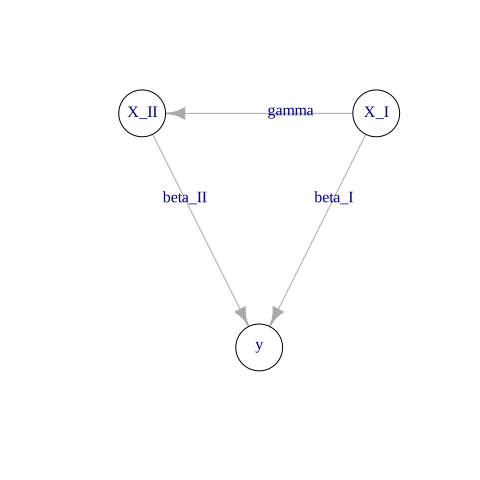
Figure 3.5: The direct and the indirect effects
In more detail, if \(\gamma=0\) then \(X_I\) does not affect at all \(X_{II}\) (they are orthogonal), hence the restricted estimates in (3.53) will be \(\widehat\beta_R=\widehat\beta_I\). That is, unlike the restricted model in which \(\widehat\beta_R\) represents the total effect of \(X_I\) on the dependent variable \(y\), \(\widehat\beta_I\) in the unrestricted model represents only the direct effect isolated from the indirect effect that comes via \(X_{II}\).
The result of (3.53) explains why not wise to regress the dependent variable on each regressor separately by a simple linear regression model because, in such an estimated model, the regression coefficient of the regressor encompasses the direct effect of that regressor with those of all the omitted relevant regressors, which is not what we may want. That is why multiple linear models are preferred since they provide every single effect isolated from the others.
For residuals, it is beneficial to compare the two residual vectors of the restricted and the unrestricted model respectively \(e_R\) and \(e\), so using (3.50), we have:
\[\begin{align*} \underbrace{M_Ie_R}_{e_R}&=M_Iy-\underbrace{M_IX_I}_{=0}\widehat\beta_R\\ e_R&=M_I(X_I\widehat\beta_I+X_{II}\widehat\beta_{II}+e)\\ e_R&=\underbrace{M_IX_I}_{=0}\widehat\beta_I+M_IX_{II}\widehat\beta_{II}+\underbrace{M_Ie}_{=e}\\ e_R&=M_IX_{II}\widehat\beta_{II}+e \end{align*}\]
The sum of squared errors of the restricted model \(e_R^te_R\) will be then:
\[\begin{align} e^t_Re_R&=(M_IX_{II}\widehat\beta_{II}+e)^t(M_IX_{II}\widehat\beta_{II}+e)\notag\\ &=\widehat\beta_{II}^tX^t_{II}M_IX_{II}\widehat\beta_{II}+\widehat\beta_{II}^tX^t_{II}\underbrace{M_Ie}_{=e}+\underbrace{e^tM_I}_{=e^t}X_{II}\widehat\beta_{II}+e^te\notag\\ &=\widehat\beta_{II}^tX^t_{II}M_IX_{II}\widehat\beta_{II}+\widehat\beta_{II}^t\underbrace{X^t_{II}e}_{=0}+\underbrace{e^tX_{II}}_{=0}\widehat\beta_{II}+e^te\notag\\ e^t_Re_R&=\widehat\beta_{II}^tX^t_{II}M_IX_{II}\widehat\beta_{II}+e^te \tag{3.54} \end{align}\]
Since \(M_I\) is a positive semi-definite matrix, the first member of the right-hand side is positive \(\widehat\beta_{II}^tX^t_{II}M_IX_{II}\widehat\beta_{II}\geqslant 0\), and hence \(e^t_Re_R \geqslant e^te\). However, the two sums are equal if \(\widehat\beta_{II}=0\).
The interpretation of the above expression is that deleting variables from the estimated model always increases the sum squared of errors, or at least never decreases. Therefore, if this increase is significant, so the omitted variables are relevant, and hence it will be worthwhile to include these variables in the model. Some statistical tests can be used in such situations to test that significance.
In case when \(\widehat\beta_R\) is unbiased (when \(\gamma=0\)), then using (3.52), the variance will be:
\[\begin{align*} Var(\widehat\beta_R)&=E\big[(\widehat\beta_R-\widehat\beta_I)(\widehat\beta_R-\widehat\beta_I)^t\big]\\ &=E\big[(X^t_IX_I)^{-1}X^t_I\varepsilon\varepsilon^tX_I(X^t_IX_I)^{-1}\big]\\ &=(X^t_IX_I)^{-1}X^t_I\underbrace{E(\varepsilon\varepsilon^t)}_{=\sigma^2I}X_I(X^t_IX_I)^{-1}\\ &=\sigma^2(X^t_IX_I)^{-1}\underbrace{X^t_IX_I(X^t_IX_I)^{-1}}_{=I}\\ &=\sigma^2(X^t_IX_I)^{-1} \end{align*}\]
Then, the estimated variance will be:
\[\begin{equation} \widehat{Var}(\widehat\beta_R)=s^2_R(X^t_IX_I)^{-1} \tag{3.55} \end{equation}\]
Where \(s^2_R=\frac{e_R^te_R}{n-(k-\mathrm g)}\).
Further, in this chapter, we will prove that this variance is less than that of the classical unrestricted model. That is:
\[\begin{equation} \widehat{Var}(\widehat\beta_R)\leqslant \widehat{Var}(\widehat\beta_I) \tag{3.56} \end{equation}\]
Example 3.3 Using the above example again, we will fit a model that includes only the first three variables \(X_2\), \(X_3\), and \(X_4\) (excluding \(X_5\), \(X_6\)) to verify the formula (3.53).
As explained above, each column in the matrix \(\gamma\) is the estimates resulted from regressing the associated regressor in the excluded matrix \(X_{II}\) on all the included regressors in the model. for our specific example, the variables of that formula have the following dimensions:
\[\begin{equation*} \underset{(4,1)}{\widehat\beta_R}=\underset{(4,1)}{\widehat\beta_I}+\underset{(4,2)}{\gamma}\underset{(2,1)}{\widehat\beta_{II}} \end{equation*}\]
The \(\widehat\beta_I\) and \(\widehat\beta_{II}\) have been already computed and are in the table 3.7.
beta_I <- tidy(mod_R_full)[1:4,1:2]$estimate
beta_II <- tidy(mod_R_full)[5:6,1:2]$estimate
list("beta_I"=beta_I , "beta_II"=beta_II)
[out] $beta_I
[out] [1] 17.454710 2.476346 -1.504809 4.924499
[out]
[out] $beta_II
[out] [1] 3.448502 5.603644The \(\gamma\) matrix, however, will be computed as follows:
# regress X5 on (X2,X3,X4)
mod_R_gamma1 <- lm(x5~x2+x3+x4, data=small_data)

# regress X6 on (X2,X3,X4)
mod_R_gamma2 <- lm(x6~x2+x3+x4, data=small_data)

# put the two vectors in a matrix
gamma <- cbind(tidy(mod_R_gamma1)$estimate,tidy(mod_R_gamma2)$estimate)
gamma
[out] [,1] [,2]
[out] [1,] 57.366141241 51.99472466
[out] [2,] 0.002563165 0.06825118
[out] [3,] 0.173194419 0.30364164
[out] [4,] 0.031965875 0.36386739We are now ready to compute the right-hand side of that formula \(\widehat\beta_I+\gamma\widehat\beta_{II}\).
[out]             [,1]
[out] [1,] 506.6418861
[out] [2,]   2.8676407
[out] [3,]   0.7939523
[out] [4,]   7.0737166
Now let us verify that result with the estimates \(\widehat \beta_R\) of the restricted model:
[out] [1] 506.6418861 2.8676407 0.7939523 7.0737166As we see, the estimates are the same, and we can check therefore the unbiasedness of the restricted estimates by inspecting the significance of each estimators vector in \(\gamma\) using F-test
| statistic | p.value |
|---|---|
| 0.3906232 | 0.7607266 |
Since F-test value is very small (and very large p-value), we can conclude that \(X_5\) is orthogonal to the included regressors (\(X_2\), \(X_3\), \(X_4\)).
| statistic | p.value |
|---|---|
| 1.692692 | 0.1930748 |
Similarly, the \(X_6\) is also orthogonal to the included regressors. However, we are not surprised by these results since our variables have been randomly and separately generated so that the orthogonality is implicitly specified, which is unlikely to happen in real data.
That said, we can say that the estimators of the restricted model, in our case, are unbiased. However, as discussed earlier, with such a model, the estimators are not efficient. We can easily verify that by comparing the standard errors between the restricted and the unrestricted model.
compar <- tidy(mod_R_full)[1:4,c(1,3)]
compar$std.error.restricted <- tidy(mod_R_restricted)$std.error
compar| term | std.error | std.error.restricted |
|---|---|---|
| (Intercept) | 7.4209844 | 86.528462 |
| x2 | 0.0981670 | 1.795375 |
| x3 | 0.0699867 | 1.198810 |
| x4 | 0.0892612 | 1.567968 |
As shown, the standard errors of the restricted model are larger than those of the unrestricted one.
The estimates of the unrestricted model.
mod_py_full = smf.ols('y~x2+x3+x4+x5+x6', data=small_data_py).fit()
summ_py_full = mod_py_full.summary2().tables[1]
summ_py_full| Coef. | Std.Err. | t | P>|t| | [0.025 ] | ||
|---|---|---|---|---|---|---|
| Intercept | 17.454710 | 7.4209844 | 2.352075 | 0.0272093 | 2.138551 | 32.770869 |
| x2 | 2.476346 | 0.0981670 | 25.225841 | 0.0000000 | 2.273740 | 2.678953 |
| x3 | -1.504809 | 0.0699867 | -21.501367 | 0.0000000 | -1.649254 | -1.360363 |
| x4 | 4.924499 | 0.0892612 | 55.169539 | 0.0000000 | 4.740273 | 5.108725 |
| x5 | 3.448502 | 0.0797868 | 43.221477 | 0.0000000 | 3.283831 | 3.613174 |
| x6 | 5.603644 | 0.0691031 | 81.091031 | 0.0000000 | 5.461022 | 5.746265 |
Retrieve the estimates of \(\beta_I\) and \(\beta_{II}\).
beta_I_py = mod_py_full.params.iloc[:4].values
beta_II_py = mod_py_full.params.iloc[4:].values
print(f'beta_I_py: {beta_I_py}\nbeta_II_py: {beta_II_py}')
[out] beta_I_py: [17.45471017 2.47634635 -1.50480863 4.92449902]
[out] beta_II_py: [3.44850235 5.60364354]The estimates of the restricted model
mod_py_restricted = smf.ols('y~x2+x3+x4', data=small_data_py).fit()
beta_R_py = mod_py_restricted.params.values
print(f'beta_R_py: {beta_R_py}')
Compute \(\gamma\).
# regress X5 on (X2,X3,X4)
mod_py_gamma1 = smf.ols('x5~x2+x3+x4', data=small_data_py).fit()

# regress X6 on (X2,X3,X4)
mod_py_gamma2 = smf.ols('x6~x2+x3+x4', data=small_data_py).fit()

# put the two vectors in an array
gamma_py = np.vstack((mod_py_gamma1.params.values,mod_py_gamma2.params.values))

# compute the restricted estimates from the formula
# and put everything in a pandas data frame
restricted_py = pd.DataFrame({'From the formula':beta_I_py+(gamma_py.T@beta_II_py),
'From the restricted model': beta_R_py,
'coefficients': ['intercept', 'X2','X3', 'X4']}).set_index('coefficients')
restricted_py| From the formula | From the restricted model | |
|---|---|---|
| intercept | 506.6418861 | 506.6418861 |
| X2 | 2.8676407 | 2.8676407 |
| X3 | 0.7939523 | 0.7939523 |
| X4 | 7.0737166 | 7.0737166 |
3.8.3 Including irrelevant regressors
Let \(X_*=[XZ]\) be a \(n\times (k+\mathrm g)\) matrix of the estimated model, where \(X\) contains the same \(k-1\) regressors (plus a vector of ones for the constant term) such as the DGP model, and \(Z\) contains \(\mathrm g\) additional irrelevant regressors. The DGP model still written as \(y=X\beta+\varepsilon\), and its corresponding estimated model with the same matrix \(X\) still also written \(y=X\widehat\beta+e\). However, if we estimate a model with the matrix \(X_*\) that includes the additional \(\mathrm g\) regressors \(Z\), this model then will be written as follows:
\[\begin{align*} y&=X_*\widehat{\beta_*}+e_*\\ &=[XZ] \begin{pmatrix} \widehat {\beta_{1*}}\\ \widehat {\beta_{2*}} \end{pmatrix} +e_* \end{align*}\]
\[\begin{equation} y=X\widehat {\beta_{1*}}+Z\widehat {\beta_{2*}}+e_* \tag{3.57} \end{equation}\]
Where \(\widehat {\beta_{1*}}\) is the coefficients vector of the DGP regressors in \(X\), and \(\widehat {\beta_{2*}}\) is the coefficients vector of the irrelevant regressors in \(Z\).
As the irrelevant regressors have no effects on the dependent variable \(y\) in the DGP model, so we expect their OLS coefficients to be non significantly different from zero. Typically, we are more interested in whether the additional irrelevant variables in the estimated model will affect or not the statistical properties of the relevant regressor estimators denoted \(\widehat {\beta_{1*}}\), the upper subset of the vector \(\widehat{\beta_*}\).
The OLS estimators vector of (3.57) will be:
\[\begin{equation} \widehat{\beta_*}=\big(X^t_*X_*\big)^{-1}X^t_*y \tag{3.58} \end{equation}\]
to check the unbiasdness , we can include the irrelevant variables in the matrix \(Z\) in the DGP equation by setting the vector of their coefficients \(\beta_{2*}\) equal to zero as follows:
\[\begin{align*} y&=X\beta+\varepsilon\\ &=X\beta+Z\overbrace{\beta_{2*}}^{=0}+\varepsilon\\ &=[XZ] \begin{pmatrix} \beta\\ \beta_{2*}=0 \end{pmatrix}\\ y&=X_*\beta_*+\varepsilon \end{align*}\]
It turns out that this expression is the same such as the first case, where the DGP and the estimated model has the same set of regressors, and since it is proved there that the OLS estimators vector is unbiased, so we get:
\[\begin{align*} &E(\widehat{\beta_*})=\beta_*\\ &E\begin{pmatrix}\widehat{\beta_{1*}}\\\widehat{\beta_{2*}}\end{pmatrix}=\begin{pmatrix}E(\widehat{\beta_{1*}})\\E(\widehat{\beta_{2*}})\end{pmatrix}=\begin{pmatrix}\beta\\\beta_{2*}=0\end{pmatrix} \end{align*}\]
That means that the OLS estimator \(\beta_{2*}\) is unbiased, so we can conclude that including irrelevant variables in the estimated model does not affect the unbiasedness of the coefficient estimators of the relevant ones.
We have shown earlier that the estimated restricted model, with fewer regressors, is more efficient than the unrestricted estimated one, even that all the regressors of the latter are significant. So it is clear that adding more regressors with nonsignificant effects will reduce the efficiency of the model. In brief, the estimators of the relevant regressors in a model that includes other irrelevant regressors are not efficient.
In practice, we do not know the DGP model, so it will be hard for the investigator for many reasons to correctly determine the required regressors. That is why the cases discussed above can occur frequently:
- In the case of the restricted model, the estimators are not unbiased (unless the included regressors and the omitted ones are orthogonal), but the model provides efficiency.
- In the case of irrelevant regressors, the estimators still unbiased but inefficient.
These results show that the investigator should trade-off between adding more variables to obtain unbiased estimators, but not efficient, and deleting more variables to obtain efficient estimators, but not unbiased.
Example 3.4 In this example, we will add two new variables to the estimated model, but since we have a large number of regressors (compared to the small sample size of 30), we will increase our sample size to 60.
set.seed(122)
# select a random sample with 60 observations
medium_data <- sample_n(my_data, 60)

# add two random variables to the data
set.seed(133)
medium_data$X7 <- rnorm(30, 12, 7)
medium_data$X8 <- rnorm(30, 19, 4)

# fit the model
mod_R_included <- lm(y~., data=medium_data)
tidy(mod_R_included)| term | estimate | std.error | statistic | p.value |
|---|---|---|---|---|
| (Intercept) | 4.0286849 | 8.5108347 | 0.4733595 | 0.6379379 |
| x2 | 2.5866885 | 0.1070955 | 24.1530989 | 0.0000000 |
| x3 | -1.5266676 | 0.0585298 | -26.0836019 | 0.0000000 |
| x4 | 4.7428771 | 0.1031431 | 45.9834445 | 0.0000000 |
| x5 | 3.6813113 | 0.0797810 | 46.1426803 | 0.0000000 |
| x6 | 5.6447233 | 0.0602042 | 93.7596697 | 0.0000000 |
| X7 | -0.0404593 | 0.0738495 | -0.5478615 | 0.5861312 |
| X8 | 0.1666501 | 0.1065444 | 1.5641374 | 0.1238513 |
By looking at the p-value column, all the explanatory variables are significant except for the new added irrelevant variables that have larger p-values \(p-value(X_7)=0.5861312\) and \(p-value(X_8)=0.1238513\).
The following script will check the efficiency of the estimated model with the added variables.
# fit the right model
mod_R_right <- lm(y~.-X7-X8, data=medium_data)
compare_results <- tidy(mod_R_right)[, c(1,3)]
compare_results$std.error.included <- tidy(mod_R_included)[1:6, c(3)]$std.error
colnames(compare_results)[2] <- 'std.error.right'
compare_results| term | std.error.right | std.error.included |
|---|---|---|
| (Intercept) | 8.3730532 | 8.5108347 |
| x2 | 0.1012808 | 0.1070955 |
| x3 | 0.0580857 | 0.0585298 |
| x4 | 0.1022321 | 0.1031431 |
| x5 | 0.0795870 | 0.0797810 |
| x6 | 0.0601461 | 0.0602042 |
As expected, the results are in line with what said earlier, larger models tend to be less efficient. The standard errors of the estimated model with the irrelevant variables included are slightly larger than those of the model with the right regressors.
Since we are using statistical terms such as correlation↩︎